
Real-Estate Price Indexes Availability, Importance, and New Developments
Edición: Vol.7 Núm.1 enero-abril 2016

|
House price indexes (HPIs) while important to the analysis of recessions are prone to methodological and coverage differences. These differences can undermine both within-country and cross-country economic analysis. The paper first examines the nature of these measurement differences and, for selected national statistical offices, illustrates measurement strategies. More formally, a panel data set of 157 quarterly HPIs from 24 countries, along with associated measurement variables, is used to report on whether and how differences in HPI measurement matter. The determinants of house price inflation are then modeled using HPIs adjusted for differences in measurement practice. onsideration is finally given to measurement problems for commercial property price indexes.
|
Los índices de precios de la vivienda (IPV), si bien son importantes para analizar recesiones, pueden verse afectados por diferencias metodológicas y de cobertura. Éstas pueden socavar el análisis económico dentro del país y de diferentes naciones. En el documento se analiza, en primer lugar, la naturaleza de estas diferencias de medición, y se presentan las estrategias de medición de algunas oficinas nacionales de estadística seleccionadas. En términos más formales, se utiliza un conjunto de datos de panel de 157 IPV trimestrales de 24 países, junto con variables de medición conexas para establecer si las diferencias en la medición del IPV son importantes y en qué medida lo son. Luego, se elabora un modelo de los factores determinantes de la inflación de precios de la vivienda utilizando IPV ajustados en función de las diferencias en la práctica de medición. Por último, se analiza el problema de medición de los índices de precios de los inmuebles comerciales. Números de clasificación JEL: C43, E30, E31, R31. Palabras clave: índices de precios de la viviendá; inflación de precios de la viviendá; índices de precios de los inmuebles residenciales. |
Recibido: 7 de enero de 2015
Aceptado: 15 de octubre de 2015
I. Introduction
Macroeconomists and central banks need mea-sures of residential property price inflation. They need to identify bubbles, the factors that drive them, instruments that contain them, and to analyze their relation to recessions.2 Such measures are also needed for the System of National Accounts and may be needed as part of the measurement of owner-occupied housing in a consumer price index —see Eurostat et al. (2013, chapter 3). Timely, comparable, proper measurement is a prerequisite for all of this, driven by concomitant data.
There have been major advances in this area foremost of which are: (i) recently developed international standards on methodology, the Eurostat et al. (2103) Handbook on Residential Property Price Indices;3 (ii) an impressive array of data hubs dedicated to the dissemination of house price indices and related series including the IMF’s Global Housing Watch; the Bank for International Settlements’ (BIS) Residential Property Price Statistics; the OECD Data Portal; the Federal Reserve Bank of Dallas’ International House Price Database; Eurostat Experimental House Price Indices; and private sources;4 and (iii) encouragement in compiling and disseminating such measures: real estate price indexes are included as Recommendation 19 of the G-20 Data Gaps Initiative (DGI), and residential property price indexes are prescribed within the list of IMF Financial Soundness Indicators (FSIs), in turn included in the IMF’s new tier of data standards, the Special Data Dissemination Standard (SDDS) Plus.5 In this paper we identify the challenges countries face in the hard problem of measuring residential property (hereafter “house”) price indexes (HPIs).6
Sections II and III cover residential property price indexes. In section II we consider some measurement issues making use of country illustrations. Compilers of HPIs are at the mercy of the limitations of data sources available to them, in terms of coverage, timeliness and methodologies they can enable, at least in the short-medium term. Our country illustrations show how differences in data sources, coverage and methods can seriously impact on country HPI measurement. A theme of section II is that compilers of official statistics can, with some patience and effort, make their own luck and such a strategy is illustrated.
Section III examines, using a more formal approach, the empirical question as to whether measurement and coverage differences for HPIs matter and the extent to which they do so as we go into recession. The importance of measurement in modeling house price inflation is also investigated.
Section IV turns to the similar, though very much harder, measurement area of commercial property price indexes (CPPIs). In this case, especially in the lead up to and during recessions, there is sparse data on very heterogeneous properties—apartments, industrial, office and retail. We briefly outline issues and some measurement devices that apply to specific statistical problems as illustrations of the complexity of work in this underdeveloped area.
II. Residential property Price Indexes: The hard Measurement problem
A. The problem
HPIs are particularly prone to methodological differences, which can undermine both within-country and cross-country analysis. It is a difficult but important area.
Critical to price index measurement is the need to compare in successive periods transaction prices of like-with-like representative goods and services. Price index measurement for consumer, producer, and export and import price indexes (CPI, PPI and XMPIs) largely rely on the matched-models method. The detailed specification of one or more representative brand is selected as a high-volume seller in an outlet, for example a single 330 ml. can of regular Coca Cola, and its price recorded. The outlet is then revisited in subsequent months and the price of the self-same item recorded and a geometric averages of its price and those of similar such specifications in other outlets form the building blocks of a CPI. There may be problems of temporarily missing prices, quality change, say size of can or sold as a bundled part of an offer if bought in bulk, but essentially the price of like is compared with like every month.7 HPIs are much harder to measure.
First, there are no transaction prices every month/quarter on the same property. HPIs have to be compiled from infrequent transactions on heterogeneous properties. A higher (lower) proportion of more expensive houses sold in one quarter should not manifest itself as a measured price increase (decrease). There is a need in measurement to control for changes in the quality of houses sold, a non-trivial task.
The main methods of quality adjustment are (i) hedonic regressions; (ii) use of repeat sales data only; (iii) mix-adjustment by weighting detailed relatively homogeneous strata; and (iv) the sales price appraisal ratio (SPAR).8 The method selected depends on the database used. There needs to be details of salient price-determining characteristics for hedonic regressions, a relatively large sample of transactions for repeat sales, and good quality appraisal information for SPAR. In the US, for example, price comparisons of repeat sales are mainly used, akin to the like-with-like comparisons of the matched models method, Shiller (1991). There may be bias from not taking full account of depreciation and refurbishment between sales and selectivity bias in only using repeat sales and excluding new home purchases and homes purchased only once. However, the use of repeat sales does not requires data on quality characteristics and controls for some immeasurable characteristics that are difficult to effectively include in hedonic regressions, such as a desirable or otherwise view.
Second, the data sources are generally secondary sources that are not tailor-made by the national statistical offices (NSIs), but collected by third parties, including the land registry/notaries, lenders, realtors (estate agents), and builders. An exception is the use of a buyer’s survey in Japan. The adequacy of these sources to a large extent depend on a country’s institutional and financial arrangements for purchasing a house and vary between countries in terms of timeliness, coverage (type, vintage, and geographical), price (asking, completion, transaction), method of quality-mix adjustment (repeat sales, hedonic regression, SPAR, square meter) and reliability; pros and cons will vary within and between countries. In the short-medium run users may be dependent on series that have grown up to publicize institutions, such as lenders and realtors, as well as to inform. Metadata from private organizations may be far from satisfactory.
We stress that our concern here is with measuring HPIs for FSIs and macroeconomic analysis where the transaction price, that includes structures and land, is of interest. However, for the purpose of national accounts and analysis based thereon, such as productivity, there is a need to both separate the price changes of land from structures and undertake adjustments to price changes due to any quality change on the structures, including depreciation. This is far more complex since separate data on land and structures is not available when a transaction of a property takes place. Diewert, de Haan, and Hendriks (2011) and Diewert and Shimizu (2013a) tackle this difficult problem.
Figure 1 shows alternative data sources in its center and coverage, methods for adjusting for quality mix, nature of the price, and reliability in the four quadrants. Land registry data, for example, may have an excellent coverage of transaction prices, but have relatively few quality characteristics for an effective use of hedonic regressions, not be timely, and have a poor reputation. Lender data may have a biased coverage to certain regions, types of loans, exclude cash sales, have “completion” (of loan) price that may differ from transaction price, but have data on characteristics for hedonic quality adjustment. Realtor data may have good coverage, aside from new houses, data on characteristics for hedonic quality adjustment, but use asking prices rather than transaction prices.
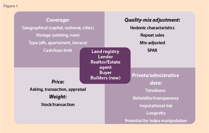
The importance of distinguishing between asking and transaction prices will vary between countries as the length of time between asking and transaction varies with the institutional arrangements for buying and selling a house and the economic cycle of a country.
B. Country illustrations9
Figure 2 shows a feast of HPIs available for the UK including the ONS (UK, hedonic mix-adjusted, completion price); Nationwide and Halifax (both UK, hedonic, own mortgage approvals, mortgage offer price; Halifax weights); the England and Wales (E&W) Land Registry (E&W, repeat sales, all transaction prices); and the ONS Median price index unadjusted for quality mix—given for comparison.10 Other available HPIs in the UK are LSL Acadata HPI (Land registry),11 Rightmove (realtor) and two HPIs based on surveys of expert opinion. Measured inflation in 2008Q4 coming into the trough was -8.7 (ONS) -12.3 (Land registry) -16.2 (Halifax) -14.8 (Nationwide): and -4.9 (ONS Median unadjusted (for quality mix change); methodology and data source matter.
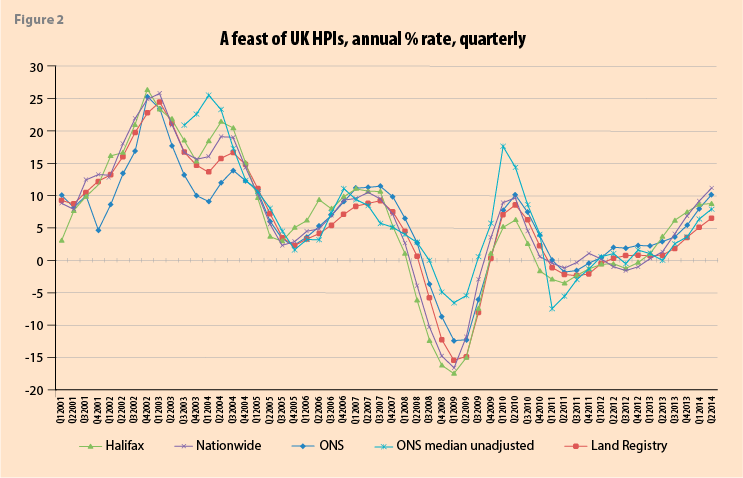
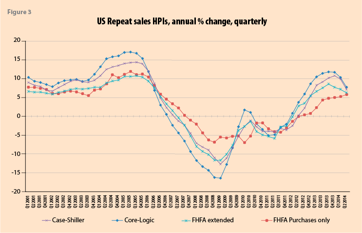
Figure 3 shows HPIs available in the US including the: CoreLogic, Federal Housing Finance Agency (FHFA) purchases-only, Case-Shiller, and the FHFA extended-data HPI. CoreLogic, FHFA, and Case-Shiller, the three primary HPIs in the US, use repeat sales for quality-mix adjustment—the Census Bureau is a (hedonic) new houses only index based on a limited sample. The FHFA extended-data HPI includes, in addition to transaction prices from purchase-money mortgages guaranteed by Fannie Mae and Freddie Mac, transactions records for houses with mortgages endorsed by the Federal Housing Administration (FHA) and county recorder data licensed from CoreLogic, appropriately re-weighted to ensure there is no undue urban over rural bias. This change in source data coverage accounted for the
4.6 percentage point difference in 2008 Q4 between the annual quarterly HPI respective falls of 6.89 and 11.66 percent for the FHFA “All Purchases” and “Extended-Data” FHFA HPIs. Coverage limited to particular types of mortgages matter.12
Leventis (2008) decomposed into methodological and coverage differences the average difference between the FHFA (then Office of Federal Housing Enterprise Oversight (OFHEO)) and S&P/Case-Shiller HPIs, covering 10 matched metropolitan areas, for the four-quarter price changes over 2006Q3-2007Q3. Among his findings was that of the overall 4.27 percent average difference, FHFA’s use of a more muted down-weighting of larger differences in the lags between repeat sales,13 than use in Case-Shiller, accounts for an incremental 1.17 percent of the difference. It is not just that the use of different quality-mix adjustment methods matters, it does also the manner in which a method is applied.
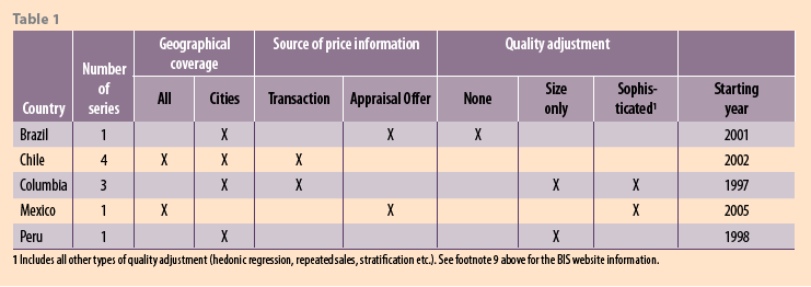
RPPIs for Latin America are reported on the BIS website, though are noted by BIS to be rather limited compared to Europe and North America. The following table is given on the BIS site to summarizes the residential property price developments in five countries in the region. Of note is the variability in the number of RPPIs, their coverage, source of price information, method of quality adjustment and longevity of the series (table 1).
C. Making your own luck
There is no need to simply accept data sources with associated problems; you can make your own luck. France benefited from the combination of a research-based central statistical agency and a monopolistic network of notaries, 4,600 in 2009. Notaries in France verify the existence of property rights, draft the legal sale contract and deed, send the records to the Mortgage Register (Conservation des Hypothèques), collect the stamp duty on behalf of the government, and send the transaction price to the tax authorities. Up to the end of the 1990s, only the “Notaires-INSEE” 1983 apartments’ index for the city of Paris was based on such data, though it was not quality-mix adjusted.14 In 1997, the National Union of Notaries (Conseil Supérieur du Notariat, CSN) and INSEE, decided to create a price index for dwellings located outside the Paris region, in the so-called Province. INSEE provided the (hedonic) technical framework. The notaries collect the data and compute the indexes at their own cost. Gouriéroux and Laferrère (2009, page 208) note that as of 2009, most contracts are still paper documents, and they are not written in the same fashion all over the country. The information must be standardized and coded. Each of the notaries is asked to send for key-boarding an extract or a photocopy of the sale deed, plus some extra information on the dwelling characteristics.
Currently, for Paris and separately for the Provinces,15 there are hedonic quality-mix adjusted HPIs for apartments and houses by about 300 zones comparing transaction prices of fixed bundles of observed characteristics. The hedonic coefficients are now updated every 2 years —previously 5 years— and weights chain-linked (Gouriéroux and Laferrère, 2009).16
The United Kingdom Office for National Statistics (ONS) developed its own independent official HPI in 1969, rather than relying on the then two major existing main HPIs compiled from loan information by two major building societies. The ONS index started in 1969 from a 5 percent sample of mortgage transactions: “…a number of building societies”. From 1993 the coverage was extended to include all mortgage lenders —between 1993 and 2002 a monthly sample of 2–3,000 transactions. In 2003 the 5 percent sample from each lender increased to 100 percent; from mid-2003 to August 2005 the sample was of about 25,000 monthly mortgage completions, increasing by end-of 2005 to about 40,000, through 2006 to 2007 to about 50,000, and in 2007 from about 60 main lenders. There was then some fall-off with the recession: in the six months to May 2010, the sample of 23,000 transactions per month was from 32 lenders. In 2011: the sample included 65-70 percent of all completions. Pre-2003 mix-adjustment used a potential of 300 cells; post-2003: 100,000 potential cells.
III. Residential property Price Indexes: More formally: An Empirical Exercise As to Why Measurement Matters
HPI measurement differences may arise from: (i) the method of enabling constant quality measures for this average (repeat sales pricing, hedonic approach, mix-adjustment through stratification, sale price appraisal ratio (SPAR); (ii) type of prices (asking, transaction, appraisal); (iii) use of stocks or flows (transactions) for weights; (iv) use of values or quantities for weights; (v) use of fixed or chained weights; aggregation procedure; (v) geographical coverage (capital city, urban etc.), (vii) coverage by type of housing (single family house, apartment etc.); and (viii) vintage, new or existing property.
A. More formally
Silver (2012) collected 157 HPIs from 2005:Q1 to 2010:Q1 from 24 countries with, for each HPI, explanatory measurement and coverage variables (details are given in Annex 1 of Silver (2012).17 The explanatory measurement variables were:
Based on coverage:
• Vintage (benchmarked on both new and existing dwellings).
New (newly constructed dwelling) = 1 (0 otherwise); Xsting (existing dwelling) = 1 (0 otherwise).
Capital (major) city = 1 (0 otherwise); Big cities = 1 (0 otherwise); Urban areas = 1 (0 otherwise); Notcapital = 1 (0 otherwise); Rural = 1 (0 otherwise).
Based on method:
• Quality-mix adjustment (benchmarked on price per dwelling, no adjustment). Hedonic regression-based = 1 (0 otherwise); Repeat sales = 1 (0 otherwise); SPAR = 1 (0 otherwise); MixAdjust = 1 (0 otherwise); SqMeter = 1 (0 otherwise).
• Wquantity = 1 (0 otherwise); Wsqmeter = 1 (0 otherwise); Wpopulation = 1 (0 otherwise); Wprice in base-period = 1 (0 otherwise).
The above panel data had fixed-time and fixed-country effects; the estimated coefficients on the explanatory measurement variables were first held fixed and then relaxed to be time varying. Subsequently, the explanatory variables were interacted with the country dummies.
First, Table 2 shows that given only measurement-related variables are included, the regressions have substantial explanatory power, , at about 0.45 in mid-2009. The result is especially notable given only fixed effects, and measurement variables were included with neither hedonic variables nor structural explanatory variables to explain house price inflation by means of supply and demand (and financing) of a country’s housing market as in, for example, Muellbauer and Murphy (2008).18 From the results of Table 3, column 2, measurement matters and, in particular, increases over the period of recession, when it really matters.
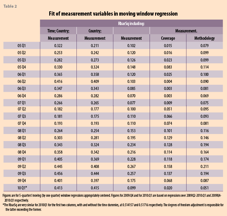
Second, Table 2 also shows the explanatory power of the model is not exclusively driven by the fixed time and cou effects. On excluding the country- and time-fixed effects, Table 3 column 4, the effect of the measurement variables alone, while diminished, accounted during the recession for about a quarter of the variation in house-price inflation rates.
Third, regarding the question: given that measurement matters, what matters most, coverage variables or methodological variables? Table 2, columns 5 and 6 find that dropping either set leaves the other with substantial explanatory power, though “method” is for the large part slightly more important than “coverage”.19
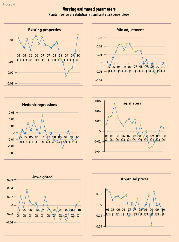
Figure 4 illustrates the nature, magnitude and volatility of individual regression coefficients over time for six
illustrative explanatory variables: the coverage of properties (as against new and existing); use of stratified mix-adjustment (as against price per dwelling); hedonic regressions (as against price per dwelling); price per sq. meter (as against per dwelling); unweighted or equal weights (as against value shares), appraisal (as against transaction) price data. A lighter-fill marker in Figure 4 indicates that the coefficient’s value is statistically significant from zero at a 5 percent level, though this has less meaning when actual (population) inflation is near zero. The general pattern is one of a substantively different (lower) effect of these variables on measured inflation during the recession compared with prior to it. There is, in some cases, a marked volatility to the effects of these variables, as illustrated in Figure 4 for the use of appraisal prices as against transaction prices.
Having shown that measurement issues matter when comparing HPIs, and that they matter particularly during the recession —when they do—we turn to a consideration of the impact of these findings on some macroeconomic analytical work.
B. The impact of measurement on modelling?
There is naturally much concern in the literature with the duration of housing cycles (Bracke (2011) and the relationship between (real) house price booms and banking busts including.
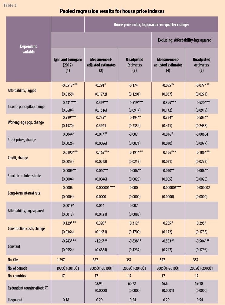
Igan and Loungani (2012), Crowe et al. (2011); and Claessens et al. (2010), though see Leamer (2007). Empirical work is often based on a sample of countries20 and includes analysis of the cross-country coincidence of real house price index changes, the magnitude, duration, and characteristics of house price cycles, and cross-country relationship between HPI changes and those of other macroeconomic and household financial variables. Implicit in such analysis is the assumption that the measurement-related differences in house price indexes between countries are not of a nature/sufficient magnitude to adversely affect the results. We take (an earlier version of) the model in Igan and Loungani (2012) (hereafter IL) to illustrate the impact of measurement differences on such analytical work. We stress that their estimates and ours are not directly comparable. Their estimates are from a regression using (unbalanced) pooled quarterly HPIs from 17 countries over 1970Q1 to 2010Q1. This contrasts with ours in a shorter period of 2005:Q1 to 2010Q1 and use of a panel data set of about 150 HPI series over a similar, but extended, set of 21 countries. Country house price inflation for our work is estimated using 441 (21 countries by 21 quarterly changes) coefficients on country-time interaction dummy variables, from a pooled regression that includes measurement variables, and time-varying country effects. However, we employ the same estimator (OLS with robust standard errors), variable list, and dynamics used by IL. We adopt their model but estimated with our measurement-adjusted or standardized HPIs —the residuals from the regression of HPIs on measurement variables— and unadjusted HPIs on the left hand side.
Table 3, column 1 provides from the results by IL from their pooled regression —further details and rationale for their model are given in IL. Quite similar results are found from our analysis given in columns 2 and 3 of Table 3 with the expected signs on the estimated coefficients. Given the quite major differences in the data sets used here and by IL, this study gives further credence to their work. Affordability is not statistically significant at a 5 percent level, but becomes so (columns 4 and 5) when its square is dropped.21
The measurement–adjusted (Madj) estimates in columns 2 and 4 improve on the unadjusted ones in columns 3 and 5. Table 3 shows both stock price changes and long-term interest rates have no (statistically significant at a 5 percent level) affect on HPI changes both for the IL estimates (column 1) and unadjusted estimates (columns 3 and 5), but do so with the appropriate sign for the measurement-adjusted estimates (columns 2 and 4).22 For some cases, parameter estimates for Madj price-changes have larger falls and smaller increases than their unadjusted counterparts. For example, Madj and unadjusted house price inflation are estimated to fall by 8.5 and 7.7 percent respectively as (lagged) affordability increases by 1 percent, to increase by 0.40 and 0.52 percent respectively as the change in income per capita increases by 1 percent, and to increase by 0.156 and 0.186 percent respectively as the change in credit increases by 1 percent.
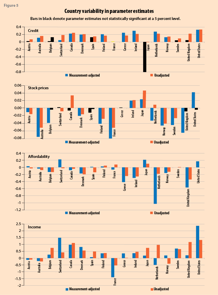
One issue of interest to this study, and also cited and explored by IL, is the cross-country variability in the parameter estimates. In Figure 5 we show the result of relaxing the restriction that the 8 estimated parameters are constant across the 17 countries, for both measurement-adjusted and unadjusted HPIs. The individual results are for the large part —over 70 percent of the 272 estimates— statistically significant at a 5 percent level. Of note is that while stock price changes and long-term interest rates were not statistically significant when related to the unadjusted measure of housing inflation in the restricted model, Table 4, these country-specific estimates were found to be generally statistically significant when allowed to vary across countries, Figure 5. The nature and extent of the country effect differed across series. For stock prices, affordability, and long-term interest rates there is evidence of larger falls when measurement-adjusted HPIs are used, while for other variables the impact of measurement-adjustment is mixed. The disparity between the estimated parameters arising from using measurement-adjusted and unadjusted HPIs, as well as the magnitude of their effects, can be quite marked in some countries, including Japan, Netherlands, Switzerland, the United Kingdom and the United States.
IV. Commercial property price indexes (CPPIs)
A. Alternative data sources: problems
The compilation of commercial property price indexes (CPPIs) is the elephant in the room. The economic analysis and modeling of HPIs is extensive as is the concern directed to the impact of house price bubbles (along with equities) on recessions. However, commercial properties can similarly be subject to bubbles and have an impact on recessions. While estimated year-end 2103 current cost of net capital stock of nonresidential fixed assets (office, retail, manufacturing and lodging) structures—though land is excluded—in the US at $1,125.8 billion was much smaller than that of private household residential fixed assets, at $15,625.9 billion, it was by no means trivial (estimates from US Bureau of Economic Analysis). Commercial properties include offices, retail, industrial, and residential (owned or developed for commercial purposes) properties. Within each of these categories, properties can be highly heterogeneous and transactions infrequent, more so than for residential, thus complicating comparisons of average transaction prices for a fixed-quality bundle of properties over time. Even where matched (repeat) transactions can be used, the population of properties sold more than once in the period of the index can be very limiting and unrepresentative of the total population of commercial properties. Kanutin (2013) highlights some of these limitations in work by the European Central Bank’s (ECB) Working Group on General Economic Statistics (WGGES) that includes results for experimental quarterly indicators for CPPIs for the EU, the euro area and 13 individual countries.
The database used for the measurement of commercial property price indexes (CPPIs) dictates the potential weaknesses in the resulting indexes and limitations of the methods available for measuring the indexes. Two major types of data are appraisals of the value of properties and recorded transaction prices. Appraisal (valuation) indexes are based on judgment, smooth and lag transaction prices and, for the large part, have serious problems with regard timeliness and representativity.23 Transaction-based CPPIs may have sample selectivity bias and limited sample sizes for these heterogeneous properties. For some countries the problem of limited samples sizes will be too severe to derive reliable CPPIs. For others, there is a need to seek methodological improvements to CPPI measurement on sparse transaction price data for heterogeneous properties. If appraisal data are to be used, there is the need of major improvements to the periodicity and concepts and operationalized measures, and a harmonization thereof, as well as further research on statistical methods of linking transaction to appraisals information, as employed by ECB on experimental transaction-linked indexes. The focus of our work is on better ways of handling transaction data —see also Bokhari and Geltner (2012), Devaney and Diaz (2011), Picchetti, Paulo (2013). More research is needed for the use of both transaction and appraisal-based data for CPPI measurement. The current data and methodological state of play is arguably inadequate for a definitive CPPI Handbook.
Two illustrations of technical research work to improve measurement are given below. Real estate price indexes are generally derived from the estimated parameters of regression models. This is necessary to repeat sales and some forms of hedonic quality adjustment. While aggregation issues in an index number context have been largely solved Diewert (1976, 1978) and the CPI Manual, ILO et al. (2004, chapters 15-20), there is little work on weighting within regressions, Diewert (2005) being an exception. We outline some such developments from Silver and Graf (2014), by necessity technical given the largely regression-based formulation of these real estate indexes.
B. Sparse data and index aggregation in a regression framework
CPPI country measurement practice, for the large part, benefits from a regression-based framework, as is the case with HPIs. Regression-based frameworks enable:
Data:
The transaction-based CPPIs used in this US study were provided to the authors by Real Capital Analytics (RCA CPPI).24 The coverage includes relatively high-value transactions; from 2000 commercial repeat-sale property transactions of over $5 million but extended in 2005 to transactions over $2.5 million (at constant dollars inflation-adjusted to December 2010). Applied filters exclude “flipped” properties (sold twice in 12-months or less), transactions not at arm’s-length, properties where size or use has changed, and properties with extreme price movements (more than 50 percent annual gain/loss).
The empirical work uses two panel data sets: RCA CPPIs from 2000:Q1 to 2012:Q4 for “apartments” broken down by 34 metros/markets areas, and similarly for “other properties” that include industrial, office, and retail —hereafter “core commercial”— properties. RCA estimates each of the 34 granular series using repeat-sales regressions. In each section below, results will be presented for both apartments and core commercial properties.
C. How to derive more efficient estimates given sparse data
The concern is with sparse data and, akin to normal statistical practice when faced with limited sample sizes, increasing the efficiency of the estimator. Geltner and Pollakowski (2007, page 18) note that the RCA National All-Property CPPI averaged 285 monthly repeat sales in 2006, but only 29 in 2001, at its inception. We use data on “counts” —number of transactions— in each quarter for each area/type of property, provided by RCA, to improve the efficiency of the estimates of US commercial property price inflation.
Consider a two-way fixed effects panel model:
![]()
where ![]() is a
is a ![]() vector of commercial property price inflation (log-change of the index) for each of the periods
vector of commercial property price inflation (log-change of the index) for each of the periods ![]() is the
is the ![]() parameter vector of spatial (area) fixed effects and
parameter vector of spatial (area) fixed effects and ![]() the associated
the associated![]() dummy variable matrix;
dummy variable matrix; ![]() is the
is the ![]() parameter vector of fixed time effects and
parameter vector of fixed time effects and ![]() the associated
the associated ![]() dummy variable matrix; and
dummy variable matrix; and ![]() are
are ![]() stochastic disturbances. The fixed time effects parameters
stochastic disturbances. The fixed time effects parameters ![]() are estimated using the least squares dummy variable (LSDV) method as opposed to demeaning, given a specific interest in
are estimated using the least squares dummy variable (LSDV) method as opposed to demeaning, given a specific interest in ![]() and inflation estimates derived therefrom; the restriction is imposed that
and inflation estimates derived therefrom; the restriction is imposed that ![]() and a constant is included in equation (1). In addition, “counts data”
and a constant is included in equation (1). In addition, “counts data” ![]() , are the number of observed price transactions for each area
, are the number of observed price transactions for each area ![]() in each period
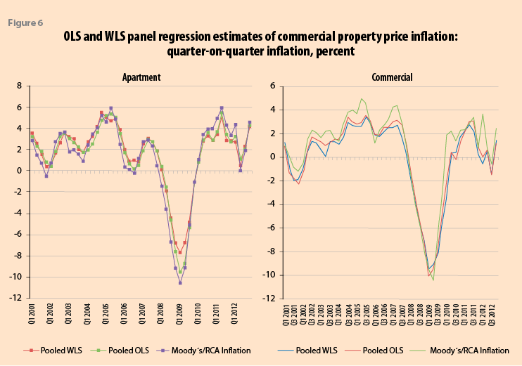
in each period ![]() . We use ordinary least squares (OLS) and weighted least squares (WLS) estimators, the latter with
. We use ordinary least squares (OLS) and weighted least squares (WLS) estimators, the latter with ![]() as explicit weights.
as explicit weights.
The assumption is that ![]() ; as counts increase, the variance decreases. The
; as counts increase, the variance decreases. The ![]() form the basis of estimates of property price inflation. Taken as a whole series, the more efficient WLS estimates can be argued to better estimate changes in commercial property price inflation. OLS gives less precisely-measured observations (more influence than they should have) and more-precisely measured ones (too little influence). WLS using counts data assigns a weight to each observation that reflects the uncertainty of the measurement and thus improves the efficiency of the parameter estimates.
form the basis of estimates of property price inflation. Taken as a whole series, the more efficient WLS estimates can be argued to better estimate changes in commercial property price inflation. OLS gives less precisely-measured observations (more influence than they should have) and more-precisely measured ones (too little influence). WLS using counts data assigns a weight to each observation that reflects the uncertainty of the measurement and thus improves the efficiency of the parameter estimates.
This focus on the efficiency of the estimator is in line with the literature on “errors in measurement” in the dependant variable —Hausman (2001). Such measurement errors result in OLS parameter estimates that are unbiased, but inefficient, with reduced precision and associated lower t-statistics and ![]() . (This differs from the literature on measurement errors in the explanatory variable for which OLS parameter estimates are biased.) The measured value of
. (This differs from the literature on measurement errors in the explanatory variable for which OLS parameter estimates are biased.) The measured value of ![]() is the sum of the true measure
is the sum of the true measure ![]() plus a measurement error
plus a measurement error![]() :
:
![]() and the true measure is
and the true measure is ![]() .
.
Instead of estimating: , ![]() we estimate:
we estimate:
![]()
Measurement error thus increases the variance of the error term from var![]() to var
to var![]() + var
+ var![]() and the variance (standard error) of
and the variance (standard error) of ![]() accordingly increases. We directly target the var
accordingly increases. We directly target the var![]() component with explicit WLS counts weights
component with explicit WLS counts weights ![]() .
.
We use all 34 area inflation rates to constitute ![]() on the left-hand-side of equation (1) above. The results are given in Figure 6.
on the left-hand-side of equation (1) above. The results are given in Figure 6.
D. How to aggregate in regression frame-work: modeling spatial dependency
The aggregate index price changes in this illustration were the parameter estimates on the time dummy used for the index estimates. This formulation for measuring aggregate price change can be subject to omitted variable bias if there are price spillovers across geographical areas. A spatial autoregressive (SAR) term is included in the regression thus removing potential bias by incorporating spillover effects —a SAR model.
Modeling spatial dependency is not uncommon in the context of hedonic house price models, for example, Anselin (2008). We include a (first order) spatial autoregressive term in equation (1), a SAR model:25
![]()
where ![]() is a
is a ![]() row-standardized spatial physical proximity weight matrix, outlined later, for the spatial autoregressive term and
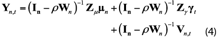
row-standardized spatial physical proximity weight matrix, outlined later, for the spatial autoregressive term and ![]() the spatial autoregressive parameter to be estimated. Equation (3) expressed in its reduced form is given by:
the spatial autoregressive parameter to be estimated. Equation (3) expressed in its reduced form is given by:
The matrix of partial derivatives of ![]() with respect to a change in a dummy time variable, is given by Elhorst (2010) and Debarsy and Ertuur (2010) as:
with respect to a change in a dummy time variable, is given by Elhorst (2010) and Debarsy and Ertuur (2010) as:

There is a resulting matrix ![]() for the marginal effect of each estimated parameter on a time dummy variable. It is apparent from equation (5) that in a fixed effect panel OLS model where
for the marginal effect of each estimated parameter on a time dummy variable. It is apparent from equation (5) that in a fixed effect panel OLS model where ![]() , the diagonal elements would be
, the diagonal elements would be ![]() and the non-diagonal effects zero, resulting in a single parameter estimate
and the non-diagonal effects zero, resulting in a single parameter estimate ![]() for each period
for each period ![]() . In this SAR model, the spatial direct effects are not
. In this SAR model, the spatial direct effects are not ![]() , but are given for each area
, but are given for each area ![]() by the diagonal elements of
by the diagonal elements of ![]() . The top-left element would be the effect on property price inflation of moving from one quarter to the next for say, Boston, but differs from the OLS estimate in that it includes the resulting feedback effects from proximate spatially dependent areas, arising from Boston’s property price inflation. Direct effects can be seen from equation (5) to depend on (i) their proximity to other areas, as dictated by
. The top-left element would be the effect on property price inflation of moving from one quarter to the next for say, Boston, but differs from the OLS estimate in that it includes the resulting feedback effects from proximate spatially dependent areas, arising from Boston’s property price inflation. Direct effects can be seen from equation (5) to depend on (i) their proximity to other areas, as dictated by ![]() ; (ii) the strength of spatial dependence,
; (ii) the strength of spatial dependence, ![]() ; and (iii) the parameter
; and (iii) the parameter ![]() . The diagonal elements are estimates of the direct effect for each area
. The diagonal elements are estimates of the direct effect for each area ![]() .
.
The indirect effects for each area ![]() are given by the off-diagonal column elements of
are given by the off-diagonal column elements of ![]() and the total effect for area
and the total effect for area ![]() is the column sum of area
is the column sum of area ![]() and includes its direct and indirect effect. We follow LeSage and Pace (2009), and the output of standard software in this area, in reporting, for the marginal effect of each time dummy parameter estimate, one direct effect as the average of the diagonal of the elements,
and includes its direct and indirect effect. We follow LeSage and Pace (2009), and the output of standard software in this area, in reporting, for the marginal effect of each time dummy parameter estimate, one direct effect as the average of the diagonal of the elements, ![]() and one total effect measured as the average of the column sums; the indirect effect is deduced as the difference between the two. The average total effect answers the question: what will be the average total impact on property price inflation of the typical area? (LeSage and Pace, 2009).
and one total effect measured as the average of the column sums; the indirect effect is deduced as the difference between the two. The average total effect answers the question: what will be the average total impact on property price inflation of the typical area? (LeSage and Pace, 2009).
The spatial approach ameliorates omitted variable bias by its inclusion of ![]() in equation (5). Debarsy and Ertur (2010), in a study of spillovers in a panel regression for 24 OECD countries of domestic savings on investment found, for 1971-1985, the coefficient from a conventional fixed effect panel estimator to be reduced from 0.609 to 0.452 when using a SAR model, a more reasonable estimate
in equation (5). Debarsy and Ertur (2010), in a study of spillovers in a panel regression for 24 OECD countries of domestic savings on investment found, for 1971-1985, the coefficient from a conventional fixed effect panel estimator to be reduced from 0.609 to 0.452 when using a SAR model, a more reasonable estimate ![]() priori in the context of the Feldstein-Horioka (1980) paradox.
priori in the context of the Feldstein-Horioka (1980) paradox.
Introducing weights
The derivation of estimates of the direct effects as an average of the diagonals and total effects as an average of the column sums of equation (5) has an interesting useful index number application. The averaging applied by the software is unweighted over ![]() the areas. We can deconstruct equation (5) into the total and direct effect for their
the areas. We can deconstruct equation (5) into the total and direct effect for their ![]() components and apply weights to the estimated area (direct and total) price changes; the weights may be relative values of the stock of, or transactions in, commercial property. Diewert (2005) previously proposed weighting systems within a regression framework via analytic weights using a WLS estimator. If using a SAR model, the framework advocated here provides an alternative explicit weighting mechanism that can be applied to each of the direct, total, and indirect spatial effects; thus, allowing WLS weights to be used for other purposes, say in relation to heteroscedasticity. For example, while the average unweighted direct effect for
components and apply weights to the estimated area (direct and total) price changes; the weights may be relative values of the stock of, or transactions in, commercial property. Diewert (2005) previously proposed weighting systems within a regression framework via analytic weights using a WLS estimator. If using a SAR model, the framework advocated here provides an alternative explicit weighting mechanism that can be applied to each of the direct, total, and indirect spatial effects; thus, allowing WLS weights to be used for other purposes, say in relation to heteroscedasticity. For example, while the average unweighted direct effect for ![]() , the weighted average of direct effects for
, the weighted average of direct effects for ![]() is given by:
is given by:
![]()
where S is a ![]() matrix whose diagonal is the area
matrix whose diagonal is the area ![]() relative shares (weights) in stocks or transactions of commercial property.
relative shares (weights) in stocks or transactions of commercial property.
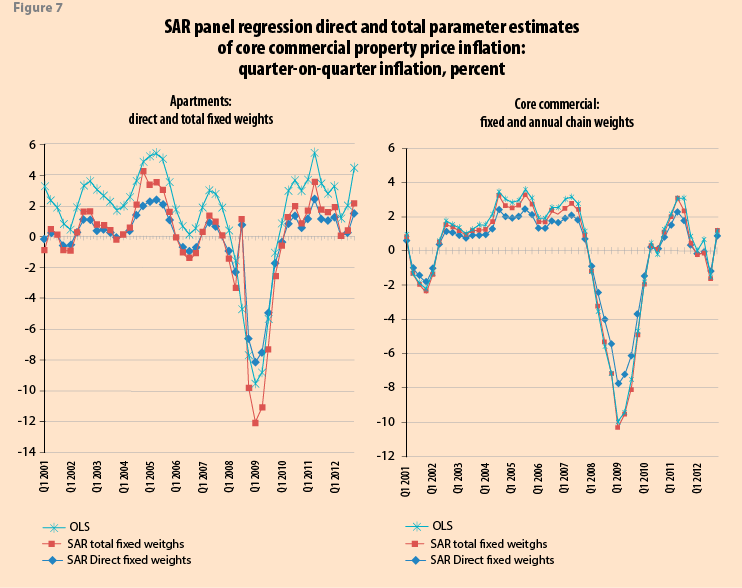
Figure 7 shows the SAR total (fixed ![]() and
and ![]() ) effect is primarily constituted by the direct effect, with little indirect difference, except for the trough in 2009. The OLS estimates are biased upwards against the SAR total (fixed) for apartments (core commercial) by, on average 1.78 (1.68) percentage, and in 2009:Q1 by 2.47 (2.48) percentage points. In Silver and Graf (2013) we relax the restriction on fixed weights.
) effect is primarily constituted by the direct effect, with little indirect difference, except for the trough in 2009. The OLS estimates are biased upwards against the SAR total (fixed) for apartments (core commercial) by, on average 1.78 (1.68) percentage, and in 2009:Q1 by 2.47 (2.48) percentage points. In Silver and Graf (2013) we relax the restriction on fixed weights.
Relaxing the restrictions of constant ![]() and
and ![]()
In empirical work both ![]() and
and ![]() are generally held constant over time. Indeed the software noted and used in Section III for spatial econometric estimation does not allow any such variation within a panel. This restriction is relaxed by annually estimating equation (5) for 4 quarters in 2000, again for 2001, 2002… 2012, thus allowing
are generally held constant over time. Indeed the software noted and used in Section III for spatial econometric estimation does not allow any such variation within a panel. This restriction is relaxed by annually estimating equation (5) for 4 quarters in 2000, again for 2001, 2002… 2012, thus allowing ![]() and
and ![]() fixed for quarters within each year, but allowed to vary between years. The results are compared in Silver and Graf (2013).
fixed for quarters within each year, but allowed to vary between years. The results are compared in Silver and Graf (2013).
V. Summary
For the hard problem of properly measuring residential-property-price-indexes countries generally have available to them secondary data sources, including land registries/notaries, lenders, realtors, buyers, and builders. Each of these sources may have different problems of coverage, pricing concept, timeliness, reliability and sufficiency for enabling quality-mix adjustment; harmonization is not a given. Looking at country illustrations we found that measurement matters when coverage is restricted and even for the manner in which a given quality adjustment method is applied. However, we also showed examples of countries making their own luck and improving their HPIs by adopting long-run strategies: the way forward.
A formal analysis showed that measurement mattered, and that it really matters when it matters, as we moved into, during and recovering from recession. It also mattered in modeling, but less so than may be envisaged.
The really hard area of price index measurement was for commercial property where transaction data can be very sparse and properties very heterogeneous. Valuation data and methodological issues for transaction-based CPPIs need both further research and development. CPPI measurement using transaction data is quite technical; two problems looked at were of sparse data and aggregation within a regression framework.
![]()
References
Akerlof, George A. and Robert J. Shiller 2009. Animal Spirits: How Human Psychology Drives the Economy And Why It Matters for Global Capitalism, Princeton University Press, Princeton NJ: March.
Anselin, L. 2008. Errors in variables and spatial effects in hedonic house price models of ambient air quality. Empirical Economics 34, 1, 5-34.
Bokhari, Sheharyar and David Geltner 2012. Estimating real estate price movement for high-frequency tradable indexes in a scarce data environment, Journal of Real Estate Finance and Economics 45, 2, 522-43.
Bracke, Philippe 2011. How long do housing cycles last? A duration analysis for 19 OECD countries, IMF Working Paper Series WP11/231 October.
Carless, Emily 2011. Reviewing house price indexes in the UK. Paper presented at the Workshop on House Price Indexes, Statistics Netherlands, The Hague, 10-11 February 201. Available at: http://www.cbs.nl/en-GB/menu/organisatie/evenementen/HPIworkshop/presentations/default.htm.
Claessens, Stijn, Giovanni Dell’Ariccia, Deniz Igan, and Luc Laeven 2010. Cross-country experiences and policy implications from the global financial crisis, Economic Policy 25, 267-293.
Crowe, Christopher, Giovanni Dell’Ariccia, Deniz Igan, and Rabana Paul 2011. How to deal with real estate booms: lessons from country experiences, IMF Working Paper Series WP/11/91.
Debarsy, Nicolas and Cem Ertur 2010. Testing for spatial autocorrelation in a fixed effects panel data model, Regional Science and Urban Economics 40, 453-470.
Devaney, Steven and Roberto Martinez Diaz 2011. Transaction Based Indices for the UK Commercial Real Estate Market: An Exploration using IPD Transaction Data, Journal of Property Research 28, 4, 269-289.
Diewert, W. Erwin 1976. Exact and superlative index numbers, Journal of Econometrics 4, 114-145.
_______ 1978. “Superlative index numbers and consistency in aggregation, Econometrica 46, 883-900.
_______ 2005. Weighted country product dummy variable regressions and index number formulae, Review of Income and Wealth 51, 561-70.
Diewert, W. Erwin, Jan de Haan and Rens Hendriks 2011. Hedonic Regressions and the decomposition of a house price index into land and structure components, Department of Economics Discussion Paper 11-01, The University of British Columbia.
Diewert, W. Erwin, and Chihiro Shimizu 2013a. A conceptual framework for commercial property price indexes, Department of Economics Discussion Paper 13-11, The University of British Columbia.
_______ 2013b. Residential property price indexes for Tokyo, School of Economics Discussion Paper 13-07, The University of British Columbia; forthcoming Macroeconomic Dynamics.
Diewert, W. Erwin, Saeed Heravi, and Mick Silver 2008. “Hedonic imputation indexes versus time dummy hedonic indexes”. In W. Erwin Diewert, John Greenlees, and Charles R. Hulten eds. Price Index Concepts and Measurement, NBER, Chicago: University of Chicago Press, 278-337, 2010.
Elhorst, J. Paul 2010. Applied Spatial Econometrics: Raising the Bar, Spatial Economic Analysis 5, 1, March.
Eurostat, European Union, International Labor Organization, International Monetary Fund, Organisation for Economic Co-operation and Development, United Nations Economic Commission for Europe, The World Bank 2013. Handbook on Residential Property Prices Indices RPPIs, Luxembourg, European Union.
Feldstein, Martin and Charles Yuji Horioka 1980. Domestic saving and international capital flows, Economic Journal 90, 314-29.
Geltner, David and Jeffrey Fisher 2007. Pricing and index considerations in commercial real estate derivatives, The Journal of Portfolio Management 33, 5, 99-118.
Geltner, David and Henry Pollakowski 2007. A set of indexes for trading commercial real estate based on the Real Capital Analytics Transaction Prices Database, MIT Center for Real Estate Working Paper, Release 2.
Gouriéroux, Christian and Anne Laferrère 2009. Managing hedonic housing price indexes: the French experience, Journal of Housing Economics 18, 206-213.
Hann, Jan de and W. Erwin Diewert 2013. Hedonic regression methods, and Jan de Hann, Repeat sales methods. In Eurostat et al. 2013 op. cit.
Hausman, J. 2001. Mismeasured variables in econometric analysis, problems from the right and problems from the left. Journal of Economic Perspectives 15, 4, 57-67.
Heath, Robert 2013. Why are the G-20 Data Gaps Initiative and the SDDS Plus relevant for financial stability analysis? Journal of International Commerce, Economics and Policy, 4, 3.
Hill, Robert J. 2013. Hedonic price indexes for residential housing: a survey, evaluation and taxonomy, Journal of Economic Surveys, 27, 5, 879-914, December.
Igan, Deniz and Prakash Loungani 2012. Global housing cycles, IMF Working Paper Series WP12/217 August.
Igan, Deniz and Heedon Kang 2011. Do loan-to-value and debt-to-income limits work? Evidence from Korea, IMF Working Paper Series WP/11/297, December.
http://www.imf.org/external/pubs/cat/longres.aspx?sk=25441.0.
International Labour Office ILO, IMF, OECD, Eurostat, United Nations, World Bank 2004. Consumer Price Index Manual: Theory and Practice, Geneva: ILO.
http://www.ilo.org/public/english/bureau/stat/guides/cpi/index.htm.
Kanutin, Andrew 2013. ECB progress towards a European commercial property price index. Paper presented at the 13th Ottawa Group Meeting held from 1-3 May, 2013, Copenhagen, Denmark. Available at:
http://www.dst.dk/da/Sites/ottawa-group/agenda.aspx.
Leamer, Edward E. 2007. Housing is the business cycle, NBER Working Paper Series, Working Paper 13428, NBER, Cambridge MA.
Leventis, Andrew 2008. Revisiting the differences between the OFHEO and S&P/Case-Shiller House Price Indexes: new explanations, Office of Federal Housing Enterprise Oversight, January, Available at: www.ofheo.gov/media/research/OFHEOSPCS12008.pdf.
LeSage J. P. and R. K. Pace 2009. Introduction to Spatial Econometrics. Taylor & Francis, New York, FL.
Mack, Adrienne and Enrique Martínez-García 2011. A cross-country quarterly database of real house prices: a methodological note,” by Federal Reserve Bank of Dallas, Globalization and Monetary Policy Institute Working Paper No. 99.
Manski, C. F. 1993. Identification of endogenous social effects: The reflexion problem. Review of Economic Studies 60, 531-42.
Matheson, Jil 2010. National Statistician’s Review of House Price Statistics, United Kingdom Government Statistical Services.
Muellbauer, John and Anthony Murphy 2008. Housing Markets and the Economy: the Assessment, Oxford Review of Economic Policy 24, 1, 1-33.
Office for National Statistics (ONS) 2013. Official House Price Statistics Explained, ONS April, 4.
Picchetti, Paulo 2013. Estimating and smoothing appraisal-based commercial real-estate performance indexes. Paper presented at the 13th Ottawa Group Meeting held from 1–3 May, 2013, Copenhagen, Denmark. Available at: http://www.dst.dk/da/Sites/ottawa-group/agenda.aspx.
Shiller, Robert J. 1991. "Arithmetic repeat sales price estimators", Journal Housing Economics 1, 1, 110-126.
_______ 1993. "Measuring asset values for cash settlement in derivative markets: hedonic repeated measures indexes and perpetual futures", Journal of Finance 48, 3, 911-931.
_______ 2014. S&P Dow Jones Indices: S&P/Case-Shiller Home Price Indices Methodology McGraw Hill Financial, July. http://us.spindices.com/index-family/real-estate/sp-case-shiller.
Shimizu, C., K. G. Nishimura and T. Watanabe 2010. Housing Prices in Tokyo: A Comparison of Hedonic and Repeat Sales Measures, Journal of Economics and Statistics, 230, 6, 792-813.
Silver, Mick 2012. Why house price indexes differ: measurement and analysis, IMF Working Paper WP/12/125. Forthcoming as “The degree and impact of differences in house price index measurement” in the Journal of Economic and Social Measurement, 2015.
_______ 2011. House price indices: does measurement matter?” World Economics, 12, 3, July-Sept.
_______ 2013. Understanding commercial property price indexes, World Economics 14, 3, September, 27-page 41.
Silver, Mick and Brian Graf 2014. Commercial property price indexes: problems of sparse data, spatial spillovers, and weighting, IMF Working Paper WP/14/72, Washington DC, April.
Silver, Mick and Heravi, Saeed 2007. Hedonic indexes: a study of alternative methods. In E.R. Berndt and C. Hulten eds. Hard-to-Measure Goods and Services: Essays in Honour of Zvi Griliches, pp. 235-268, NBER/CRIW, Chicago: University of Chicago Press.
![]()
1 The views expressed in this paper are those the author and do not necesarily represent the views of the IMF, its Exscutive Board, or IMF managment.
2 For salient papers see the recent Conference by Deutsche Bundesbank, the German Research Foundation (DFG) and the International Monetary Fund on “Housing Markets and the Macroeconomy: Challenges for Monetary Policy and Financial Stability” at: http://www.bundesbank.de/Redaktion/EN/Termine/Research_centre/2014/2014_06_05_eltville.html.
3 http://epp.eurostat.ec.europa.eu/portal/page/portal/hicp/methodology/hps/rppi_handbook.
4 The IMF’s Global Housing Watch provides current data on house prices for 52 countries as well as metrics used to assess valuation in housing markets, such as house price-to-rent and house-price-to´-income ratios: http://www.imf.org/external/research/housing/; the BIS has extensive country series on HPIs along with details of, and links to, country metadata and source data: http://www.bis.org/statistics/pp.htm; OECD also disseminates country house price statistics and is developing a wide range of complementary housing statistics: http://www.oecd.org/statistics/; see also the Federal Reserve Bank of Dallas’ International House Price Database, Mack and Martínez-García (2011), at: http://www.dallasfed.org/institute/houseprice/index.cfm and Eurostat Experimental House Price Indices at: http://appsso.eurostat.ec.europa.eu/nui/showdo?dataset=prc_hpi_q&lang=en.
5 The setting of such standards is a key element of Recommendation 19 of the report: The Financial Crisis and Information Gaps, endorsed at the meeting of the G-20 Finance Ministers and Central Bank Governors on November 7, 2009; see Heath (2013) for details of SDDS Plus and the DGI and http://fsi.imf.org/ for FSIs under “concepts and definitions”.
6 We draw on Silver (2011, 2012, and 2013) and Silver and Graf (2014).
7 International manuals on all of these indexes can be found at under “Manuals and Guides/Real Sector” at: http://www.imf.org/external/data.htm#guide. This site includes the CPI Manual: International Labour Office et al. (2004).
8 Details of all these methods are given in Eurostat et al. (2013); see also Hill (2013) for a survey of hedonic methods for residential property price indexes; Silver and Heravi (2007) and Diewert, Heravi, and Silver (2008) on hedonic methods; Diewert and Shimizu (2013b) and Shimizu et al. (2010) for an application to Tokyo; and Shiller (1991, 1993, and 2014) on repeat-sales methodology.
9 Data are generally sourced from: http://www.bis.org/statistics/pp.htm use also being made of: http://www.acadata.co.uk/acadHousePrices.php; http://www.ons.gov.uk/ons/rel/hpi/house-price-index/july-2014/stb-july-2014.html; http://us.spindices.com/indexfamily/real-estate/sp-case-shiller; http://www.fhfa.gov/KeyTopics/Pages/House-Price-Index.aspx; and http://www.fipe.org.br/web/index.asp?aspx=/web/indices/FIPEZAP/index.aspx.
10 A detailed account of the methodologies and source data underlying these HPIs for the UK is given in Matheson (2010), Carless (2013), and ONS (2013); see also http://www.ons.gov.uk/ons/guide-method/user-guidance/prices/hpi/index.html.
11 Acadata use a purpose built “index of indices” forecasting methodology to help “resolve” the problem that only 38 percent of sales are promptly reported to Land Registry, considered by Acadata to be an insufficient sample to be definitive. The LSL Acad HPI “forecast” is updated monthly until every transaction is included. Effectively, an October LSL Acad E&W HPI “final” result, published with the December LSL Acad HPI “forecast” is definitive.
12 http://www.fhfa.gov/PolicyProgramsResearch/Research/Pages/Recent-Trends-in-Home-Prices-Differences-across-Mortgage-and-Borrower-Characteristics-.aspx.
13 The S&P/Case-Shiller methodology materials suggest that its down-weighting is far more modest than FHFA. Over longer time periods, evidence suggests that there is greater dispersion in appreciation rates across homes. This variability causes heteroskedasticity, which increases estimation imprecision. The down-weighting mitigates the effect of the heteroskedasticity. Leventis (2008, page 3) notes that the S&P/Case-Shiller methodological material suggest valuation pairs, which reflect the extent to which homes have appreciated or depreciated over a known time period, are given 20-45 percent less weight when the valuations occur ten years apart vis-à-vis when they are only six months apart. By contrast, OFHEO’s down-weighting tends to give ten-year pairs about 75 percent less weight than valuation pairs with a two-quarter interval. Differences in filters and coverage of qualifying loans (FHFA) account for much of the rest.
14 The ‘Notaires-INSEE’ stratified quarterly index (without quality adjustment) had been computed since 1983 for second-hand apartments in Paris. INSEE defined 72 strata and provided weights from the Population Census; the index was computed by the Chambre Interdépartementale des Notaires Parisiens (CINP), the Parisian branch of the notaries.
15 The existing properties HPI for Île-de-France are calculated by the company Paris Notaires Services (PNS) and INSEE using property transaction data contained in the BIEN (Notarial Economic DataBase) database, which belongs to and is managed by PNS and funded by notaries from Île-de-France. The existing properties HPI for the provinces are calculated by the company Perval and INSEE using data from property transactions contained in the Perval database and funded by notaries from the provinces. Gouriéroux and Laferrère (2009) note that together they included some 6 million housing transactions at the end of 2008, with 30 percent of the transactions in the Ile-de-France, and 70 percent in the Province. The existing properties HPI for the whole of Metropolitan France are calculated by the company Parvel and INSEE using data from property transactions contained in the data bases managed by Perval and PNS.
16 Data are available at http://www.bdm.insee.fr/bdm2/choixCriteres?codeGroupe=1292;methodology at http://www.bdm.insee.fr/bdm2/documentationGroupe?codeGroupe=1292 and Gouriéroux and Laferrère (2009).
17 Information on the characteristics of the house price indexes was based on the methodological notes attached to the source data, survey papers, and, often, extensive email correspondence with the providing institutions. The HPIs were from: national (official and private) sources and the BIS Residential Property Price database, http://www.bis.org/statistics/pp.htm.
18 The paper finds the main drivers of house prices to include income, the housing stock, demography, credit availability, interest rates, and lagged appreciation.
19 There is likely to be some intercorrelations between the variable sets. For example, in the United States, the repeat-purchase method is used to hold constant the quality mix of transactions for existing houses, but for new houses sold only once, the hedonic method is used, since new houses (coverage) will generally have only one transaction (method). More generally, Land Registry data based on transaction prices often has a large coverage, but limited characteristic variables, arguing against the use of hedonic regressions, while the opposite applies to realtor data based on asking prices.
20 Work has also been undertaken for states within countries, for example Igan and Kang (2011) for Korea and the United States.
21 Excluded from Table 4 are the country effects (available for the authors) required by our model given that more than one series is used for each country. F-tests on the redundancy of these country effects found the null hypothesis of no such effects to be rejected at a 1 percent level (F = 3.735 and 2.887 respectively for the measurement– adjusted and unadjusted estimates).
22 The coefficient for stock prices in column (4) denoted as statistically significant at a 10 percent level was in fact a borderline p-value of 0.1056. We used a (White) period heteroscedasticity adjustment to the standard errors. Had diagonal or cross-sectional one been applied the p-value would have been 0.017 and 0.069 respectively, compared with p-values of 0.2076 and 0.1884 for the unadjusted estimates.
23 Appraisal data used for investment return indexes comprise a valuation and rental income component. There is a school of thought that the valuations over time may be used for CPPIs, along with adjustments for depreciation and capital expenditure on improvements to return the property to the preceding period’s state. The proposal arises as a solution to the problem of sparse transaction data. However, first, guidelines to professional appraisers are that they base their appraisal on the transactions of similar properties currently in the market, introducing circularity in the argument that appraisals solve the problem of sparse data. Second, in the majority of European countries, annual appraisals are the norm with linear interpolated values used to derive quarterly series: thus in any quarter, on average, one quarter of appraised prices will be based on a linear interpolation commencing a year ago and three-quarters of appraised prices will be imputed on this basis, there being no extrapolations used. (In the US, annual external appraisals are supplemented by in-house estimates by the property owners/ managers.) Third, information on capital expenditures and depreciation are used, in appraisal-based indices, as a means for quality adjustment between appraisals. There is much in the definition of these variables that render them inadequate as currently constructed for the needs of CPPIs. Fourth, guideline for appraisals and definitions vary between and within countries, and substantially so. Fifth, the sample of values is for larger professionally-managed properties—there may be a sample selectivity bias. Finally, there is evidence that appraisal-based indexes unduly smooth and lag prices Geltner and Fisher (2007).
24 We acknowledge their support both in the provision of data and ongoing advice. Information on the RCA CPPI is at: https://www.rcanalytics.com/Public/rca_cppi.aspx; see Geltner and Pollakowski (2007) for methodological details.
25 We note from Manski (1993) that when a spatially lagged dependent variable, spatially lagged regressors, and a spatially autocorrelated error term are included simultaneously the parameters of the model are not indentified unless at least one of these interactions is excluded. We found no firm evidence for the spatial autocorrelated error (SEM) model and our explanatory variables of interest, the time dummies, a priori, have no spillover effect. In any event, we follow the more general advice by LeSage and Pace (2009, pp. 155-58), and Elhorst (2010) to adopt the SAR model and exclude the spatially autocorrelated error term to favor inclusion of the spatially autoregressive one.