EPUB PDF

1. Introduction

Mexico witnessed substantial poverty reductions for over a decade (1996-2006). However, these good results were partially reverted, according to the 2008 and 2010 official reports during the international food price crisis of 2007 and the global financial crisis of 2008 and 2009. In particular, the increment in poverty for the first quintile appears to be heavily linked to the increase in food prices (Chavez et al. 2009). Nonetheless, the impoverishment around the second and third quintiles need to be further investigated. Since these two quintiles obtain most of their monetary resources from labor, a better understanding of the labor markets during this period is fundamental. A deteriorated labor market, defined as one that pays very low wages and offers reduced (or null) social protection, may cause poverty and vulnerabilities in many population groups. If this is the case, public policies should be targeted to improve the labor markets. Moreover, the identification of such exposures can help to reduce the influence of economic shocks to poverty and social welfare.

In this paper, we will address labor fragility by characterizing the jobs in the Mexican market and their evolution during the last two international crises. Even though the words “labor-market deterioration” can be understood in many different ways, we will relate them to two concepts: a) loss of social security or b) a decrease in wages. A related question is to what extent is deterioration concentrated in poor households.

The official poverty measurements in Mexico are computed using the Encuesta Nacional de Ingresos y Gastos de los Hogares (ENIGH): a sophisticated income-expenditure household survey that has many virtues, one of them being the inclusion of a large set of sociodemographic variables. Nonetheless, it presents two important caveats. The first one is that it is a cross-section survey, making the study of income dynamics difficult. The second is that, although the ENIGH distinguishes individuals’ earnings by source, a limited set of variables describes their work environment. The latter means that the labor information is not as rich and complete when compared to other specialized employment surveys. These two caveats may explain why (to the best of our knowledge) the link between poverty and labor markets in Mexico has been so scarcely documented.

Additionally, Mexico has another employment survey, a comprehensive one called Encuesta Nacional de Ocupación y Empleo (ENOE), which is a semi-rotating panel on five consecutive quarters. With the aid of econometric techniques, the dynamics of labor conditions can be depicted for some population groups.

In this project, we matched the workforce found in ENOE 2010 with its “counterparts” observed in ENIGH 2010 to identify the poor. Afterward, we matched again ENOE 2010 with ENOE 2006 to depict the market dynamics of the individuals. The overall plan is to build a synthetic master database that theoretically will preserve the strengths of both types of surveys. After we had matched the three datasets, several labor market characteristics were constructed to characterize their dynamics through the mentioned timespan. Given that we labeled households according to their poverty status and income levels, we expect this procedure will shed some light on the link between labor markets and poverty evolution in Mexico during this period.

The primary objective of the paper is to understand how labor-market conditions changed between 2006 (the last year when poverty in Mexico was reduced) and 2010 (when the economic alleviation appeared after the downturn derived from the international crises of 2007-2009) for the poorer households of Mexico (quintiles I and II). Even if we are not able to identify how each crisis affected the labor market particularly, we will be capable of depicting its evolution during the international shocks above mentioned.

This report organizes the research in the following way: the next section describes and explains the matching methodology; section 3 presents the hypotheses to be tested and their results; and finally, section 4 briefly states conclusions, and mentions some lines for further developments.

2. Double Statistical-Matching Technique

Database matching techniques have lately become relevant among researchers due to the convenience of using information that is stored in different sources, that was gathered by multiple procedures and providers, but that describe the same target population. There are three primary methodologies for joining data sets: merge, record linkage, and statistical matching (or data fusion, in Europe). The first two use unique identifiers to integrate the information. In contrast, the last one faces a lack of identifiers in databases that do not contain either the same number of variables or the same amount of observations between each other (D’Orazio et al. 2001). Hence, matching techniques use variables in common between two or more datasets to identify “similar” observations, link them, and consequently allow a better and more complete analysis than when they were in separate databases (Kum and Masterson 2008).

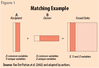
For instance, when databases do not share a unique identifier that could facilitate the joining process, a set of variables in common between databases serves as the linking bridge. To illustrate this, in the basic statistical matching methodology, let’s assume that A and B data sets share a set of variables X, while variables Y are available only in A and variables Z are only in B. In this case, the matching technique objective consists in linking A and B through the X variables in common with the goal of investigating the relationship between Y and Z (Figure 1). In this case, database A would be considered as the recipient file because it would preserve its structure and observations (unless there are some left unmatched) after the process is over. Observations from the donor file can be matched multiple times (especially when the number of records is different) or not at all. This procedure matches “statistically similar” observations and not identical ones.

To D’Orazio (2011), in the traditional statistical matching, all methods (parametric, nonparametric, and mixed) that use a common set of variables X to match A and B databases together, implicitly assume a conditional independence of Y and Z given X. This assumption is particularly strong, though it seldom holds in practice.¹

Given the structure and procedures of the surveys used, we will assume that Y (observed only in A), Z (observed only in B), and X (common in both) are multivariate random variables with a joint probability or density function.

2.1 Description of the databases

To analyze different hypotheses of deterioration in the Mexican labor market and its effects on the poor, it is convenient to have a high-quality panel data. However, there is not a single dataset with the desired properties, which drives the need to use and combine different sources. Specifically, two databases could help with the purposes of the research: Encuesta Nacional de Ingresos y Gastos de los Hogares (ENIGH), and Encuesta Nacional de Ocupación y Empleo (ENOE), both developed by the Instituto Nacional de Estadística y Geografía (INEGI).

The INEGI carries out the ENIGH every two years, and its primary goal is to obtain information about size, sources, and distribution of households’ incomes and expenditures. Also, it contains information about sociodemographic and occupational characteristics, as well as housing infrastructure and equipment. Means are representative at a national level, in rural and urban areas, and for some states.

Since 2008, the Módulo de Condiciones Socioeconómicas (MCS) has been undertaken by INEGI and the Consejo Nacional de Evaluación de la Política de Desarrollo Social (CONEVAL) as an ENIGH’s annex, with the goal to extend and satisfy the requirements of a more in-depth poverty analysis. It collects state-specific information about household incomes, family composition, health, education, social security, housing quality, basic services, and economic activities of each family member. We chose to work with this database because it offers the possibility to obtain representative results at a state level. So, from now on, when we mention the ENIGH, we will be referring to the MCS.

The ENOE have a quarterly periodicity with the goal of obtaining information about labor and occupational characteristics and other kinds of variables that allow job market analyses. The results are statistically representative at a national level, state level, some cities, and rural and urban areas. The ENOE rotates 20% of the sample in each update. In this way, the survey’s sample is continuously changed, and it is entirely renewed after 15 months.

As far as we know, while researchers widely use both surveys for poverty (ENIGH) and labor (ENOE) estimations, they have never used them together. We believe that it is important to characterize labor markets with the richness provided by ENOE and the income distribution —and, hence, the poverty categories— captured by ENIGH.

We are particularly interested in the labor dynamics in Mexico between 2006 and 2010 because 2006 was the last year when official estimations showed reduction of poverty in the country. It is crucial to policy-makers to understand the extent to which the rise in poverty could have been driven by the increase in food prices, by the deterioration of labor markets, or by any other cause.

2.2 Procedure

We chose ENOE 2010-III (third quarter) as the recipient dataset, which would be first matched with ENIGH 2010 and, afterward, again with ENOE 2006-III (third quarter). Hence, it would be a “double matching” procedure. The goal is to pair household identifiers across all three databases, know which observations can be linked together, and then choose and pick all the needed variables from these databases “on demand”.

We followed several steps in both “ENOE 2010-III—ENIGH 2010” and “ENOE 2010-III—ENOE 2006-III” matches. First, we chose and harmonized their common variables. Second, we estimated propensity scores through a probabilistic regression model by using the aforementioned variables. The use of propensity score method has the goal of finding similar households among databases, according to the probabilities obtained. Third, we developed an algorithm based on the so-called nearest neighbor matching.

2.2.1 Preparation and harmonization of databases

To match the three different databases, first we had to harmonize all their variables in common. In this case, sociodemographic variables are the best option with which to realize the statistical matching technique, since their definition among databases is the same. Moreover, these variables are deliberately built and asked for the purpose of constructing connecting vessels between databases and describing the different population segments in the country. In this way, sociodemographic variables in both surveys will establish the links between all data sources, therefore allowing analyses that will exploit the way the ENOE captures labor issues and the ENIGH gathers poverty variables.

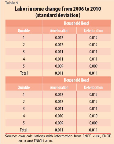
According to D’Orazio (2011), before applying statistical matching techniques, some previous procedures are required: (a) the choice of the matching variables, related to the matching methodology; (b) the proper identification of all common variables; (c) the verification that common variables are not presenting missing values as well as that all observed values are accurate; and (d) the corroboration that common variables have the same distribution (i.e. that datasets are representative samples of the same population). In this way, we chose a series of common variables in all databases, which we harmonized regarding definitions, units, and distributions. The following tables show the quality of common variables and the result of the harmonization process. We present the mean and standard deviations of the common variables to show how these are similar between databases, so as to confirm that they describe the same target population (Tables 1 & 2). Given that the ENIGH and both ENOEs surveys were built to represent the Mexican population at a national level, state level, and urban and rural areas, we will assume that the socio-demographic variables commonly found in all of them have the same distribution.

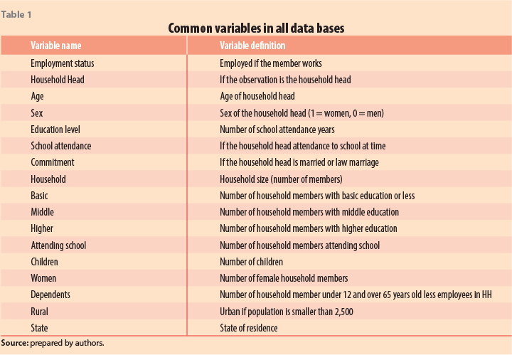
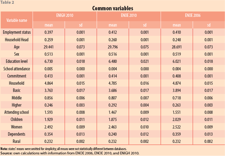
The common variables chosen were utilized to characterize three dimensions: the individual’s characteristics (age, sex, education attainment, and marital status), the household composition (education of members, the number of women, dependents, and size), and the home features (whether rural or state of residence). Each can influence positively or negatively the need, preference, or ability of an individual to be employed.

2.2.2 Propensity Score Estimation

The next step is to estimate propensity scores by using the already harmonized common variables. Studies often employ propensity score matchings where a randomized experiment is not available and when there is a need to compare a treatment group with a suitable control group. Under this methodology, both groups are matched in such a way that they only differ in the treatment received but are identical in all other characteristics (Steiner and Cook 2013). The primary advantage of this procedure is that it reduces the dimensionality problem involved in multivariate analyses into one constructed variable: the propensity score (Kum and Masterson 2008).

In our particular case, we do not have any treatment given to any group. Nonetheless, we are interested in finding comparable observations, given the common variables between the data sets. Therefore, the reduction of dimensionality that the propensity score offers will help us more easily to find “similar” records between all databases by ranking and sorting them.

Our prime interest is to analyze the labor market evolution amidst the global crises of 2007-2009. Thus, by comparing employed people from our selected databases, we will be able to depict any deterioration in their job environment or situation. Our probit model will use the employment status of the individual as its dependent variable, and the rest of the selected common variables of Tables 1 and 2 as its regressors. This procedure will rank and sort records with similar and comparable probabilities of being employed or not, according to their characteristics, household composition, and home features.

In both matches (i.e. ENOE 2010-III—ENIGH 2010 and ENOE 2010-III—ENOE 2006-III), the two databases were stacked up, and one single probit regression was computed by using observations from both sources that had 16 years or more of age. Although four years elapsed between surveys, because of limitations on the information available, we will assume that ages, marital status, educational levels, and other characteristics remained unchanged and therefore no adjustments to them were performed. The ENOE 2010-III sample size was of 279,932 respondents, the ENOE 2006-III of 318,991, and the ENIGH 2010 of 163,105. A re-weight of this synthetic data set was needed to avoid any bias that could come from each survey’s sample size and design, through which each ended with an imposed and balanced 50% post-weight.

2.2.3 Statistical Matching Algorithm

Finally, the last step of this technique is to sort the records of both surveys according to their propensity score and then search for and find the recipient’s “similar” observation in the donor data set. It would first look for its “nearest neighbor” in probability by using the Euclidean distance function³ and then link their identifiers. In this case, we imposed the restriction that the propensity scores difference between the recipient and the donor should be .05 (5% of probability) or less.⁴ Additionally, to prevent matches between logically different records (e.g. matching a “man” with a “woman”), we will have the following as “critical variables”: sex, age, if rural, and if the individual is or is not the household head.

As a result, this procedure yields multiple selections or no selection (unmatched) of donor records in the recipient database. This technique will allow us, through a simple merge among our selected databases, to construct new variables by picking the information gathered in ENIGH 2010, ENOE 2006-III and ENOE 2010-III. Initially, a 0.64% of the ENOE 2010-III’s observations ended without a counterpart from the ENIGH 2010 and a 0.35% from the ENOE 2006-III.

We bootstrapped both statistical matchings 1000 times (drawing a sample with replacement of size N from each database) and then computed our hypotheses’ means and standard errors, aiming to reduce hidden biases from the observations and the matching algorithm.⁵ Bootstrap is a nonparametric method used to test statistics by resampling data. It is very helpful when there is a random sample with an unknown distribution. When the sample size is large, the bootstrap method estimates the “true” parameters that converge by an increase in the number of repetitions. An excellent discussion of desired conditions can be found in Guan (2003), Horowitz (2001), and McKinnon (2006).

3. Results and Evidence of a Deteriorated Labor Market⁶

An understanding of the adjustments that the Mexican labor markets have forgone during economic crises is critical. A deteriorated job market, defined as one that pays low wages or that offers reduced or null social protection, may cause poverty and vulnerability in many population groups. If this is the case, public policies should be targeted to improve market conditions during these times. The proper identification and correction of such vulnerabilities can help reduce the influence of the economic shocks on overall poverty and social welfare. Using the database created, we can estimate labor situation changes in households (poor and non-poor) to see if there is any evidence of differentiated welfare damage during the aforementioned global crises.

To examine the effects of the international crises in the Mexican labor market, especially in the poorest households, we will compute different statistics. Our objective is to estimate the proportion of households and household heads that are better off, worse off, or have remained relatively unchanged in terms of employment between 2006 and 2010. We will analyze five key work attributes: labor income, health access, hours worked, formality, and employment level. Except for the latter, which uses all observations, we will only utilize those records whose household heads had a job in 2006 and 2010. This sample selection will isolate the effect of the market deterioration for working persons. The dynamics of participation in the labor market would imply a different analysis.

The labor-income evolution between 2006 and 2010 is hereby presented in real terms, using the latter as the base year. It is a numeric variable reported in both ENOEs about how much does a person earn per month. However, many zeros are present in the survey because some respondents refused to inform their figure. Only in those cases, we imputed this information through the use of a secondary question, in which the income is given through a minimum wage scale. The intervals are as follows: (1) less than 1 minimum wage (MW); (2) between 1 and 2 MWs; (3) between 2 and 3 MWs; (4) between 3 and 5 MWs; (5) above 5 MWs; (6) he/she does not receive any income; (7) not specified. So, for those who did not give a numeric answer, we used the mid-point of the interval, and the income imputations were as follows: for the first range, half MW was imputed; for the second, 1.5 MWs; for the third, 2.5 MWs; for the fourth, 4 MWs; for the fifth, 7 MWs; for the sixth, nothing was done; and for the seventh and last, the income averages across different education levels were estimated and imputed accordingly. We used their respective regional MWs.

The health variable is considered only if such benefit comes from a social security institution, such as the IMSS, ISSSTE, PEMEX, and other private systems. It does not include health access to the public health program Seguro Popular, which is not linked to an employment condition. Formality refers to individuals, who work in businesses, corporations, institutions, and societies. In contrast, informality relates to the part of the economy that is not controlled by legal regulations, such as the granting of social benefits to employees or paying taxes. The ENOE explicitly recognized this situation in one of its variables, and we used it for this purpose. We also considered domestic work and subsistence farming as informal jobs.

Results will show the statistical summaries for the household head and the household as a whole, with the information divided into quintiles. “Amelioration” considers an increase in their (individual or aggregated) labor income, in their access to social security institutions (when they did not have it before), in their hours worked, in their status change from not being employed to being employed, and in their change from informality to formality. “Deterioration” indicates when differences between the previous condition and the present decreased, and “unchanged” means no variations between the periods.

Table 3 shows that all quintiles had a reduction in their labor income; more than half of all household heads and families suffered some deterioration. The “net” column is the difference between observations that improved the labor situation and those that worsened it; this column shows that the lower quintiles were the most affected, with a slight emphasis on the third. It is worth mentioning that households’ income was reduced in a larger proportion than that of the household head. Though several hypotheses may be suggested, it seems that women’s and youths’ jobs were more deteriorated in relative terms.

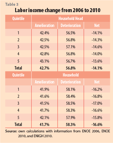
Before proceeding, some limitations of the study design should be considered. First, these numbers were taken from the ENOE survey and, as mentioned before, its income database is very limited compared to the ENIGH. Second, other types of resources were not captured, such as real estate revenues, dividends, and own business utilities, which could be crucial for many households, in particular for the upper quintiles. Third, there was a significant amount of missing income information in the ENOE. Fourth, as most surveys do, ENOE has a censored “top income”, where the richest families are not adequately sampled. Therefore, the average income-change could be smaller than the actual. Nonetheless, we are interested in gains that come from the labor market particularly, and Table 3 captures their evolution.

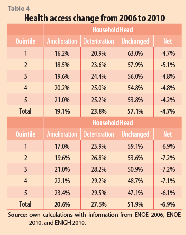
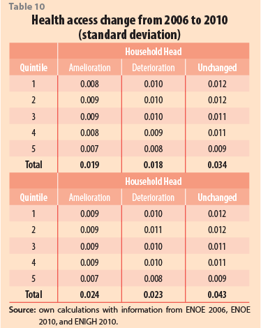
Results presented in Table 4 display that the second quintile was, overall, the most damaged between periods, regarding their employment-based health benefit. Although the dynamic was that the majority of households from all quintiles were unaffected or saw an improvement in this variable (with a figure that goes up to 70% and 80% nationally), there were between 20% and 30% who lost their access to social security institutions. This result has a direct effect on poverty and welfare, especially in our target group of study: the second and third quintiles. Nonetheless, in absolute terms, the upper quintile households had the highest deterioration (29.5%), but also the largest improvement (23.4%).

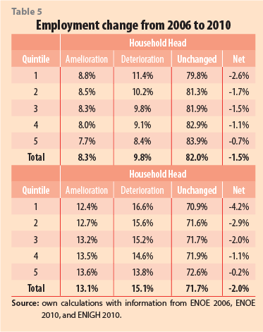
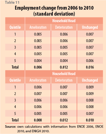
According to Table 5, changes from employment to unemployment were concentrated noticeably more in the lower quintiles. Moreover, the fifth quintile household could compensate for almost all of the deterioration suffered between periods (with a -0.2% net figure), and it ended in 2010 with about the same employment figure of 2006, which was not the case for the rest. Thus, these findings suggest that, regarding employment deterioration between the international crises, it comes especially from the poorest. For instance, a 16.6% of the first quintile household members lost their job, and only a 12.4% could reincorporate into a new one.

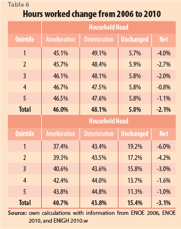
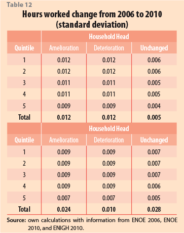
Additionally, using figures from Table 6, we can see that the lower quintiles again had the greatest loss, but now in their working hours. However, even when the household head of the first quintile was the most affected (with a 49.1% deterioration figure), this quintile was the least damaged when considering and adding the other family members’ labor (a 43.4% number). Thus, on the one hand, the poorest suffered a reduction in their working hours individually, but on the other hand, they compensated it through the work of other members, who helped the family to improve or at least to stay unchanged, in comparison with year 2006.

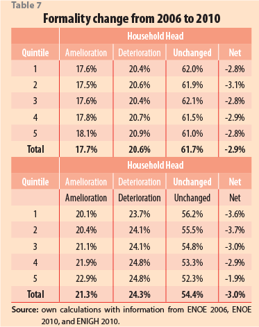
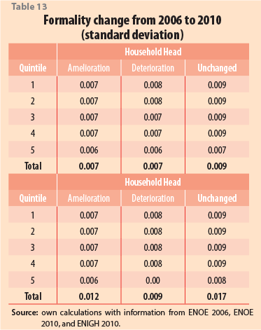
Finally, Table 7 shows that the participation dynamics of the household heads in the formal sector was relatively the same across quintiles, regarding their amelioration, deterioration, and unchanged figures. However, when compared at a household level, although the deterioration is relatively even, the amelioration is noticeably concentrated in the uppermost quintile. They moved from informal labor to formality in the largest percentage (22.9%).

So, at first glance, previous results show an overall labor deterioration in Mexico for all quintiles, with a slight concentration toward the poor. For example, when Fallon and Lucas (2002) reviewed the impact of the 1990s financial crises on the labor market, household income, and poverty level of several countries, they found that there were at least three ways to adjust labor markets—namely to cut wages, employment, or hours. In response to this, some households seem to have reduced their incomes during the shock through increasing their labor-force participation or by relying on transfers. The alternative for others was the reduction of goods’ consumption. Nonetheless, the authors concluded that the dominant impact of these crises on labor markets was a cut in real wages rather than unemployment or increases in labor schedules. However, in our findings, reductions in employment and working hours were also present during the global crises of 2007-2009, in addition to those observed in labor incomes.

In a Latin American study, Martínez and Aguilera (2009) analyzed how the economic cycles have a strong relationship with the behavior of unemployment, real wages variation, participation in the informal sector, and retirement patterns. In relation to the Mexican case specifically, Freije et al. (2011) describe how the crises increased the unemployment rate and participation in informal activities, while average real wages declined. Although we share the same findings as them, our results are differentiated across poor and non-poor households and not only through a time-series analysis.

Other notable highlights, with respect to the Mexican case, are related to the importance of social security for job retention and household protection, because unemployment increases a household’s risk of becoming poor, making it a critical or, sometimes, a vital issue (World Bank 2010). According to Fallon and Lucas (2002), as the 1994-95 crisis intensified in Mexico, job retention was much higher among protected workers (those with social security or in government employment) than unprotected workers. In this sense, Martínez and Aguilera (2009) argue that social security institutions support families in distress and prevent societies from drifting into a generalized state of indigence. Although our results cannot explicitly confirm this, we found that loss of access to healthcare and unemployment were slightly higher in the lower quintiles and, therefore, increased the household’s risk of becoming poor. Additionally, according to Cortés (1995), although the labor force of the lower quintiles in Mexico has increased, their income barely improved, given the weakening of wages in real terms. Comparably, we found that household working hours of the first quintile were the least reduced, 56.5% still saw their incomes deteriorated between 2006 and 2010.

3.1 Non-Labor Income⁷

The linkage of poverty to labor income cannot avoid its connection to another question: To what extent can less well-off households mitigate their situation with non-labor income? To a large degree, this critical angle is out of the scope of the present investigation since the master data set employed in this paper was constructed to capture labor dynamics. Nonetheless, a preliminary analysis is considered. Firstly, we will discuss the relative weight of various income sources by quintiles for both years 2006 and 2010. Secondly, together with the relative sizes of alternative sources, we will present a comparison of essential household characteristics (on income) for the year 2010. Given that we generated our poverty labels for that year, the household characteristics associated with these labels should hint some associated elements.

Before proceeding, it is necessary to highlight a critical caveat. The problem with the non-reporting of income sources, described for labor income, is much more accentuated for those with an own-business income. While the problem can concentrate more strongly on the top-income families, the effects of non-reporting are very uncertain for lower income groups. How to treat business revenues in the existing surveys is an empirical question that deserves considerable attention.

Figures 2 and 3 show the income composition of the households by quintile. The results pinpoint that the first quintile depends heavily on transfers and other sources, representing almost half of their total revenues. In contrast, for the fifth quintile, wages account for around three-quarters of their total income (Figures 2 & 3). The information comes from the ENIGH survey (for years 2006 and 2010), given that the information that ENOEs provide in non-labor income sources is very limited.

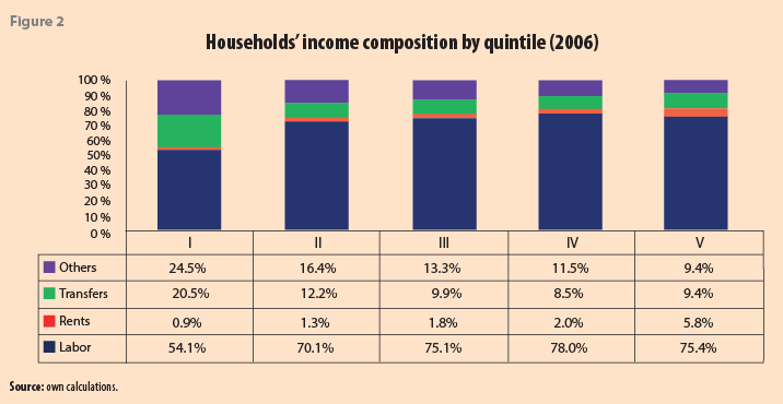
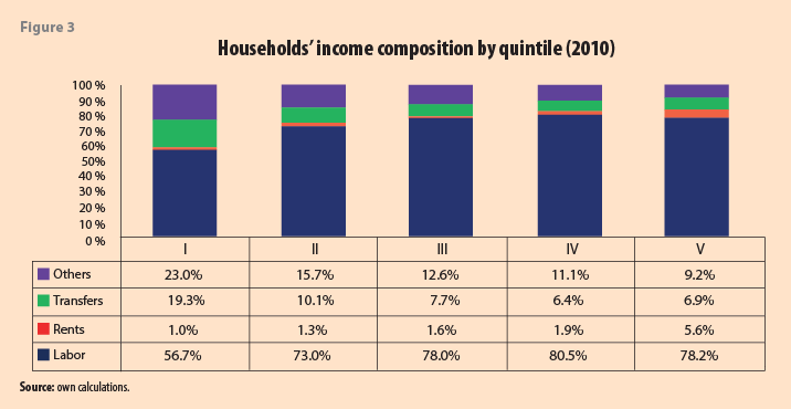
A fascinating preliminary result is that despite the crisis described in the introduction of this paper, the related structures of sources of revenue remain more or less constant between 2006 and 2010. Labor income is slightly greater, on average, in relative terms for all the quintiles. Given the labor income deterioration documented above, the indirect result that emerges suggests that non-labor income (from capital sources and transfers) suffered even more. This issue is another possible cause for the drastic increase in poverty.

In Table 8, two groups of incomes are considered. Labor income is the standard definition employed above, but is restricted to primary jobs. “Other sources of income” include rents, own business revenues (capital), and secondary jobs in case they exist. We did not consider transfers of any sort. This classification has the advantage of reflecting the households’ capacities to generate income. The association with other variables is helpful when investigating the sources of inequality.

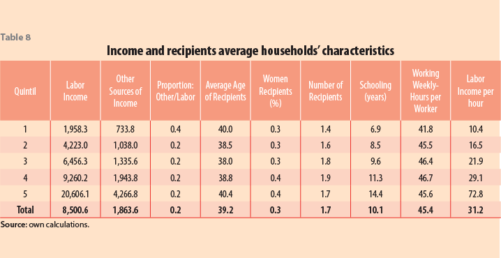
The poorest quintile has the highest income ratio on the issue of “other sources to labor”. Given their lack of capital (with transfers not taken into account), these incomes should be associated with secondary jobs and low-capital entrepreneurial activities. The ratio remains constant from the third to the fifth quintiles. While the number of recipients (persons) has its highest point in the fourth quintile, women recipients top both fourth and fifth quintiles. The school years follow a more or less linear pattern on quintiles, but labor income per hour appears very convex, thus separating the fifth quintile from the rest of the distribution. Other sources follow a similar pattern but on a lesser magnitude.

A tentative conjecture, combining both Figures 2 and 3, and Table 8, is that the poorest households may be pushed out of the labor market seeking alternative sources of income. However, if this is the case, these other sources of income have had a rather limited capacity to mitigate poverty.

4. Conclusions

This report explored to what extent the labor market deterioration in Mexico was concentrated in the poorest households between 2006 and 2010. We believed that while the increment in food prices had had a direct effect on the lowest-income groups, changes in the labor market had especially affected the second and third quintile and made them more vulnerable to become poor (or poorer). By developing and deploying a “double statistical matching” procedure, we could identify poor and non-poor households according to the income-expenditure survey, ENIGH, and construct their labor market dynamics with the aid of two employment surveys, the ENOEs, conducted at different periods. Working with a synthetic household database, we were able to shed some light on issues that were previously only assumed.

This research is pioneer in the creation of a database that was specially designed to study the phenomenon underlying the deterioration of the labor markets and its effects on the poor. Even when our results become from external sources, they are the first results that matched both labor and poverty using different data sets to analyze the implications of the former on the latter.

First, we found that there is a generalized deterioration in the labor conditions for households across the income distribution, which is not surprising if we consider the enormous crises seen between 2006 and 2010. Nonetheless, there are significant findings such as having uneven changes and favoring the upper quintiles for either increasing their income or for having more healthcare access. It was also found that even when formality broadly spreads across all quintiles, it has a higher propensity within the richest households. Similarly, it can be concluded that the lowermost quintile household heads reduced their working hours to a greater degree than the uppermost quintile, but, at the aggregate family level, they could revert this deterioration; although with no noticeable improvement in their labor income level.

It is of particular importance that formality increased in the highest quintiles and this quintile maintained relatively more healthcare access than the lower quintiles. Moreover, lower income households were more affected by losing their job than those in the uppermost quintile, which was relatively unchanged. Preliminary analyses of non-labor incomes suggest that the capacity to contend the reduction in labor income was very narrow. Thus, the increments in poverty levels are fairly consistent with incomes dynamics.

This report should help our understanding of the evolution of labor markets during crises and its implications for poverty and the poor. This understanding may also contribute to the creation of better public policies and, therefore, mitigate the effect of future crises on the poorest households. It would be valuable to expand this report to include dynamics for relevant socio-demographic variables, such as cohort, region, gender, educational level, and specific industries. Certainly, we have not exploited completely and taken full advantage of the data set we constructed; nonetheless, this first approach could still provide policymakers with useful insights about incidence in the poorest households and what aspects most critically affect the social welfare and vulnerable groups.

References

Cortés, F. (1995). “El ingreso de los hogares en contextos de crisis, ajuste y estabilización: un análisis de su distribución en México, 1977-1992”, in: Estudios Sociológicos. XIII: 37, 91-108.
Chávez, J. C., H. J. Villarreal, R. Cantú & H. González. “Impacto del incremento en los precios de los alimentos en la pobreza en México”, in: El Trimestre Económico. LXXVI (303), 775-805. 2009.
D’Orazio, M. “Statistical Matching and Imputation of Survey Data with the Package StatMatch for the R Enviroment”. The Comprehensive R Archive Network (CRAN). 2011.
D’Orazio, M., M. Di Zio, & M. Scanu. Statistical Matching: a tool for integrating data in National Statistical Institutes. Italian National Statistical Institute. 2001.
Fallon, P. & R. Lucas. “The Impact of Financial Crises on Labor Markets, Household Incomes, and Poverty: A Review of Evidence”, in: The World Bank Research Observer. 17(1), 21-45. 2002.
Freije, S., G. López-Acevedo & E. Rodríguez-Oreggia. Effects of the 2008-09 Economic Crisis on Labor Markets in Mexico. Working Paper WPS5840. World Bank. 2011.
Guan, W. “From the help desk: Bootstrapped standard errors”, in: The Stata Journal. 3(1), 71-80. 2003.
Horowitz, J. “The Bootstrap”. Handbook of Econometrics, in: J. Heckman & E. Leamer (ed.). Handbook of Econometrics. Edition 1, volume 5, chapter 52, 3159-3228 Elsevier. 2001.
Kum, H. & T. Masterson. Statistical Matching using Propensity Scores: Theory and Application to the Levy Institute Measure of Economic Well-Being. Working Paper No. 535. The Levy Economics Institute of Bard College. 2008.
Martínez, G. & N. Aguilera. Unemployment and Wages During Economic Cycles in the Americas. Working Paper No. 09022. Inter-American Conference on Social Security (CISS). 2009.
McKinnon, J. Bootstrap Methods in Econometrics. Working Paper No. 1028. Department of Economics. Queen’s University. 2006.
Rosenbaum, P. & D. Rubin. “The Central Role of Propensity Score in Observational Studies for Causal Effects”, in: Biometrika. 70(1), 41-55. 1983.
Steiner, P. M., & D. Cook. “Matching and propensity scores”, in: The Oxford Handbook of Quantitative Methods in Psychology. 1, 237. 2013.
Van Der Puttan, P., J. N. Kok & A. Gupta. Data Fusion Through Statistical Matching. Working Paper No. 185. MIT Sloan Working Paper. 2002.
World Bank. Social Impact of the Crisis and Building Resilience. Report No. 55111-HR. World Bank and UNDP. 2010.

Annexes

¹ This criterion is called the Conditional Independence Assumption (CIA). It assumes that the records in both datasets are drawn randomly and independently of each other from the same population. In other words, combining the two files is only possible if the specific variables Y and Z are conditionally independent given the common variables X = x.
² For more information about poverty measurement in Mexico visit: www.coneval.gob.mx
³ The distance function is given by:
Where is the X_ki is the K^th common variables in the recipient file (ENOE 2010-III) and X_kj is K^th the common variable in the donor file (ENIGH 2010 or ENOE 2006-III).
⁴ This required that (X_i - X_j) ≤ 0.05
⁵ There is a non-trivial issue regarding the robustness of the resulting synthetic data set with regards to the initial recipient file employed. The criterion here was to link all observations through the ENOE 2010-III since it could be considered to be at the center point of our analysis. That is, it was conducted in the same year as the ENIGH 2010, and it has the same structure as the ENOE 2006-III. Moreover, our interest was the analysis of the labor market, so it made sense to keep this specialized survey as our keystone. We thank Gabriel Martínez for making this point.
⁶ An annex at the end of this paper presents the standard deviations of both tables and results shown in this section.
⁷ We very much appreciate the discussion with Prof. Albert Berry about this issue, and related comments on previous drafts