1. Introduction

Smoothing methods for economic time series were derived in the econometrics literature for the purpose of obtaining business cycles for decision making, Burns and Mitchell (1946). The concept of trend arises naturally when carrying out statistical or econometric analysis of economic time series. This can be explained by the fact that the trend of a time series plays a descriptive role equivalent to that of a centrality measure of a data set. In addition, very often the analyst wants to distinguish between short- and long-term movements; the trend is an underlying component of the series that reflects its long-term behaviour and evolves smoothly, Maravall (1993), Heath (2012).

Hodrick and Prescott (1997) proposed a smoothing approach, known as the H-P method, that is very similar to a procedure that had been in use among actuaries called graduation, Whittaker (1923). The original method was further developed and is usually known among actuaries as the Whittaker- Henderson method. Nevertheless, the literature on smoothing methods based on their approach continued to grow separately from the graduation literature, due to the usefulness of identifying economic cycles. The H-P method requires that the researcher set the value of a particular constant, usually identified as λ, and whose specification has been somewhat arbitrary, or ad-hoc. In this paper we present a Bayesian approach in which Hodrick and Prescott's λ is obtained as a Bayesian estimator.

The Hodrick-Prescott Method

In this approach the observed time series is considered as the sum of seasonal, cyclical and growth components. Usually, however, the method is actually applied to a series that has been previously seasonally adjusted, so that this component has already been removed. Hence in their conceptual framework a given (previously seasonally adjusted) time series is the sum of a growth (or trend) component g_i and a cyclical component c_i

(1)

Their measure of the smoothness of the { g_i} path is the sum of the squares of its second difference. The c_i are deviations from g_i and their conceptual framework is that over long time periods, their average is near zero. These considerations lead to the following programming problem for determining the growth components:

(2)

In their formulation, the parameter λ is a positive number that penalizes variability in the growth component series. The larger the value of λ , the smoother the solution series is. For a sufficiently large λ, at the optimum, all the ( g_i- g_i-1 ) must be arbitrarily near some constant, β , and therefore the g_i arbitrarily near g₀+βi. This implies that the limit of solutions to program (2) as λ approaches infinity is the least squares fit of a linear time trend model.

Based on ad-hoc arguments Hodrick and Prescott arrive at a 'consensus' value that is extensively used when analyzing quarterly data (the frequency most often used for business cycle analysis): the value of λ =1600. This parameter tunes the smoothness of the trend, and depends on the periodicity of the data and on the length of the main cycle that is of interest. It has been pointed out that this parameter does not have an intuitive interpretation. Furthermore its choice is considered perhaps the main weakness of the H-P method, Maravall and del Rio (2007). The consensus value changes for other frequencies of observation; for example, concerning monthly data (a frequency seldom used), the econometrics program E-Views uses the default value 14400.

Maravall and del Rio (2007) make two important remarks:

a) Given that seasonal variation should not contaminate the cyclical signal, the HP filter should be applied to seasonally adjusted series. In addition, the presence of higher transitory noise in the seasonally adjusted series can also contaminate the cyclical signal and its removal may be appropriate.

b) It is well known that the H-P filter displays unstable behavior at the end of the series. Endpoint estimation is considerably improved if the extension of the series needed to apply the filter is made with proper forecasts, obtained with the correct ARIMA

Schlicht (2005) proposes estimating this smoothing parameter via maximum-likelihood. He also proposes a related moments estimator that is claimed to have a straightforward intuitive interpretation and that coincides with the maximum-likelihood estimator for long time series, but his approach does not seem to have had acceptance.

Guerrero (2008) proposed a method for estimating trends of economic time series that allows the user to fix at the outset the desired percentage of smoothness for the trend, based on the Hodrick-Prescott (H-P) filter. He emphasizes choosing the value of λ in such a way that the analyst can specify the desired degree of smoothness. He presents a method that formalizes the concept of trend smoothness, which is measured as a percentage. However, there is no clear interpretation of the degree of smoothness nor an objective procedure for determining the percentage of smoothness one would want in a given situation.

Bayesian Seasonal Adjustment

In a related paper Akaike (1980) proposed a Bayesian approach to seasonal adjustment that allows the simultaneous estimation of trend (trend-cycle) and seasonal component. He starts by assuming that the series can be decomposed as

(3)

where T_i , represents the trend component, S_i is the seasonal component with fundamental period p and ε_i a random or irregular component. These components can be estimated by ordinary Least Squares (OLS), if we minimize

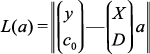
However, in seasonal adjustment procedures there are usually some constraints imposed on the T_i and S_i. On one hand there is a smoothness requirement that he imposes by restricting the sum of squares of the second order differences of T_i, that is (T_i -2_i-1+T_i-2 ), to a small value. Similarly, the gradual change of the seasonal component is imposed by requiring that the sum of square differences in the seasonal components. (S_i -S_{i-p}) be small. The usual requirement that the sum of S_i's within a period be a small number is also imposed in this manner. Thus a constrained Least Squares problem is formulated, and the following expression should be minimized:

where d,r,z are unknown constants whose values must be specified. The constrained LS problem, as stated by Akaike (1980), is then to find the M dimensional vector ɑ that minimizes

(4)

where X is an NxN matrix, α₀ is a known vector, || || denotes the Euclidean norm, and R is a positive

definite matrix. But minimizing (4) is equivalent to maximizing

where σ² is a positive constant. He points out that the constrained LS problem is equivalent to the maximization of the posterior distribution of the vector α assuming the data distribution is multivariate Normal

(5)

and the prior distribution α of , given by

(6)

Akaike (1980) assumes R=D^TD=D, where D is an LxM matrix of rank M , so that we can write

and

where its minimum is attained at

Hence we conclude that the previous solution is the posterior mean of α, whose posterior distribution is given by

(7)

If there is no seasonal component, or if has been previously removed, then the constrained LS is equivalent to the H-P method with λ=d². Under this formulation λ has a very specific meaning.

Bayesian Graduation

Because of some developments in the actuarial literature are related, de Alba and Andrade (2011), we will briefly describe the more relevant ones. Kimeldorff and Jones (1967) presented a first proposal for

Bayesian Graduation. They consider simultaneously estimating a set of mortality rates for many different ages. They point out that one (implicit) assumption that actuaries have been making is that the true mortality rates form a smooth sequence, so that graduation has traditionally been associated to smoothing. The smoothness constraint is not made explicitly.

In a more recent paper Taylor (1992) presents a Bayesian interpretation of Whittaker-Henderson graduation. The relation between Whittaker-Henderson and spline graduation is identified. He also points out similarities to Stein-type estimators. But the part relevant to this paper is the reference to the loss function. He defines a loss function (under our notation)

where Δ is the difference operator and w_i=1/Vαr(y_i). The constant c assigns relative weights to deviation and smoothness and is called the relativity constant. He indicates that one of the difficulties in this approach is the lack of theory guiding the choice of c, and that the principles according to which the selection is made are only vaguely stated. Thus the constant somehow measures the extent to which the analyst is willing to compromise adherence to the data in favor of smoothness, so that 1/ c may be viewed as the variance on a prior on whatever smoothness measure is used, usually some order of differencing.

Hickman and Miller (1978) discuss Bayesian graduation in which c is also assigned a prior distribution. Carlin (1992) presents a simple Bayesian graduation model, based on Gibbs sampling, that simplifies the problem of prior elicitation.

In the context of graduation, in the actuarial sense Guerrero et al. (2001) propose an index to measure the proportion of P in (P+ )^-1, where P and are N×N positive definite matrices. He mentions that this index was originally employed by Theil in 1963. It is given by

where tr(.) denotes trace of a matrix. This is a measure of relative precision that satisfies the following properties: (i) its values are between zero and one; (ii) it is invariant under linear nonsingular transformations, (iii) it behaves linearly and (iv) it is symmetric. From this, the index of smoothness is defined as

(8)

where K₂^´K₂ determines the precision matrix of the trend in his model. This index depends only on the values λ and N, because K₂ is fixed.

Except for Hickman and Miller (1978), in all the previous references the relativity constant c (or the relative precision h or λ) are either assumed known or assigned arbitrarily, or set to achieve a 'desired' degree of smoothness. Here we use a Bayesian formulation similar to the one given by (5)-(7). We assume that the observed values y are generated from a multivariate Normal with mean α, and precision matrix κ I_N , i.e.

and the prior distribution of the vector α is given by

To complete the specification we assign gamma priors to k and δ, and we must set α₀ equal to some known judiciously specified value. Then we let the prior precision matrix R=δD^TD, where D is chosen so that Dα is a vector of second differences, except for the first and second terms, that is

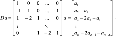(9)

The posterior distribution for the vector α can now be obtained by MCMC using WinBUGS, using as prior information the vector α₀, in the model described above. We proceed to illustrate using a real example.

An Application of Bayesian Seasonal Adjustment and Smoothing

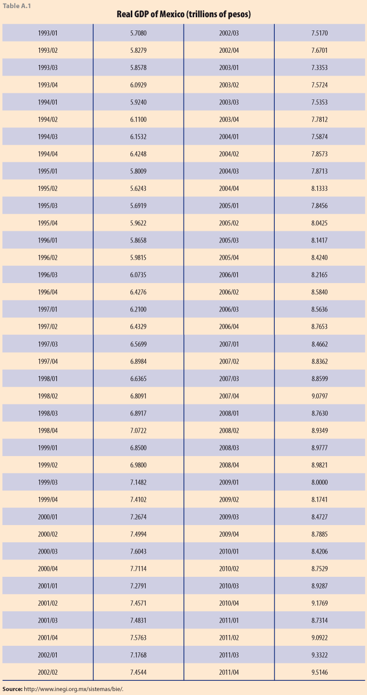
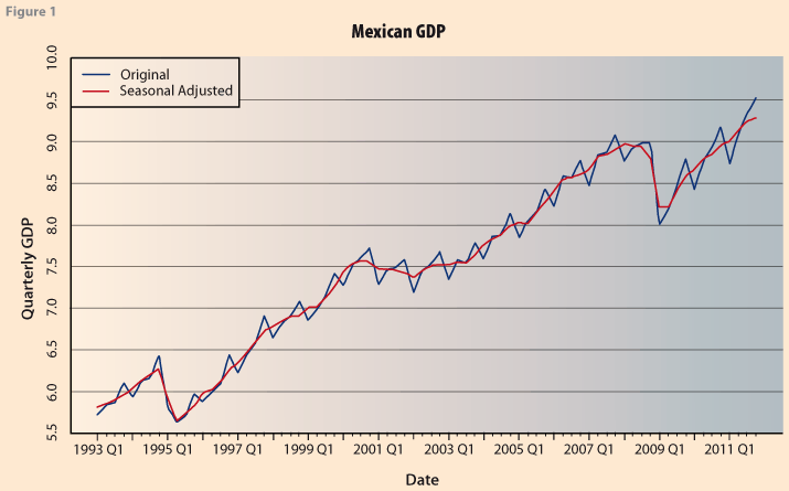
Here we use a time series of Mexican quarterly GDP, from the first quarter of 1993 to the fourth quarter of 2011, Table A.1 in Appendix 1. Figure 1 shows the original data (corrected for calendar days) and the seasonally adjusted series, as published by INEGI, see http://www.inegi.org.mx/sistemas/bie/.

The H-P filter is usually applied to seasonally adjusted data, Hodrick and Prescott (1997). However, in the Bayesian setup, if we use a model like the one proposed by Akaike (1980), this is not necessary. We first apply the Bayesian model based on this formulation, so that the exponent in (6) is

Notice that unlike Akaike's model, for simplicity, in this expression we set r = z. In particular Ꮦ²= δ²r²= δ²z².

Next, we obtained the posterior distribution for the vector of Mexican GDP and for the two parameters k and δ, assuming a-priori that k~Gα (1,0.01) and δ~Gα (1,0.001). This was done with WinBUGS. These are non-informative priors. We generated 52000 samples and dropped the first 2000 as burn in. We suggest that the mean of their posterior distributions are a natural choice for these parameters, and not ad-hoc as currently available procedures.

Figure 2 compares the estimated series. The dots represent the original unadjusted series. The one labeled INEGI shows the official seasonally adjusted (trend-cycle) series. The "linear trend" provides the prior values for the vector α. The curve labeled posterior "mean of α" provides a Bayesian estimate of the trend-cycle. Except for periods in 1994 and 2009 where there were abrupt changes, both INEGI and Bayesian are very close. The posterior means of the parameters were the following: E(k|y)=317.9, E(δ|y)=188.0 and E(Ꮦ|y)=542.7. These are estimates that minimize the expected value of a quadratic loss function with respect to the posterior distribution of the parameters. The complete distribution can be analyzed and probability statements obtained.

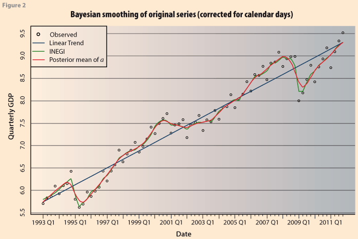
This is in contrast to the values suggested by Hodrick and Prescott (1997), who based on ad-hoc arguments arrive at a 'consensus' values. In the seasonal adjustment framework Akaike (1980) indicates that these values must be 'judiciously' chosen; and Ishiguro (1984) states they must be 'suitably' chosen. In the latter, the constant equivalent to κ is estimated by minimizing the statistic ABIC.

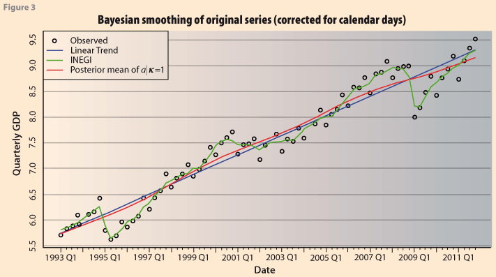
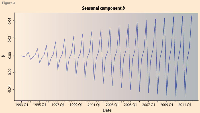
However, considering that λ=(δ|k), then, in order to make the results strictly comparable to the formulation of Akaike (1980), we now carry out the simulation with the constraint that k=1.0 Figure 3 shows the resulting series. The Bayesian trend is much smoother than before. This is in accordance with the kind of results obtained from Akaike (1980). It corresponds to the posterior mean of the vector α, and it is a Bayesian estimate of the trend of the series. Figure 4 shows the corresponding Bayesian estimates of the seasonal components. Clearly it is not a constant seasonal pattern, as might be expected from the observed behavior of the series, especially after 2009. We do not pursue this further here since it is not the purpose of the paper. In this case the posterior means of the parameters were the following: E(δ|y)=2815 and E(Ꮦ|y)=1243.9.

This example shows how the Bayesian approach to seasonal adjustment can be carried out and the estimates of the trend-cycle and the seasonal component are obtained as the posterior mean of the specified parameters.

Bayesian Analysis of the Hodrick-Prescott Filter

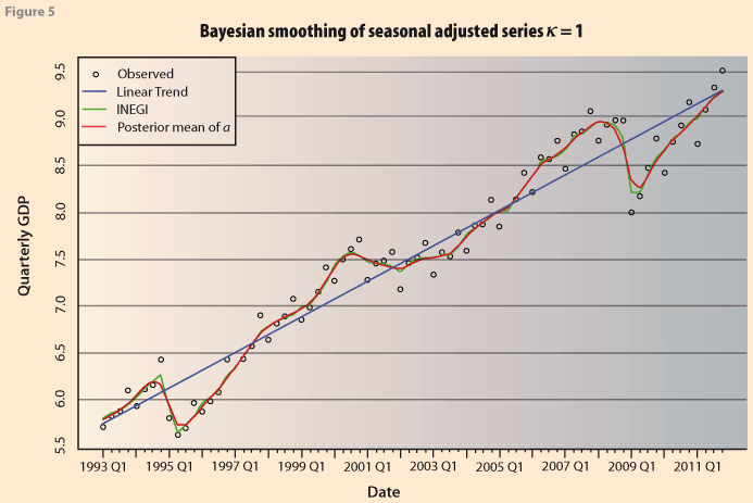
The H-P method is normally applied to series that have been previously adjusted for seasonality, so that now we apply the Bayesian model to the INEGI series without a seasonal component. This is equivalent to the Akaike procedure but leaving out the seasonal component. We apply it to the same Mexican GDP series. This will also allow us to analyze the degree of smoothness using the results of Guerrero (2008). The posterior means of the parameters are now E(δ|y)= 152 and E(k|y)= 413.8.

Figure 5 shows the resulting series from applying the Bayesian version of the H-P method. The resulting Bayesian estimate (red line) is very close to the original INEGI series. This is to be expected since it corresponds to the Bayesian estimator of a trend-cycle for the series, specifying a prior distribution for each one of the parameters, δ and k.

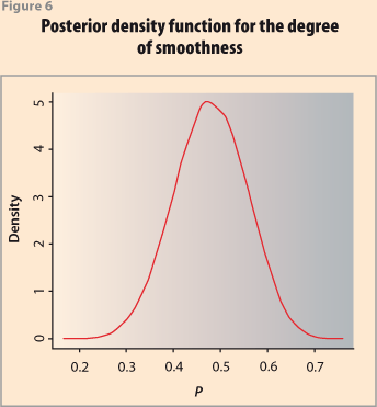
We now analyze the smoothness of the series. Under the Bayesian model, the expression for the degree of smoothness in equation (8) becomes

(10)

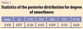
where R is the precision matrix of the prior distribution as given in (6) with R= δD^TD and D defined as in (9). Allowing for both parameters, δ and k to have a prior distribution, so that at each stage of the simulation λ=(δ|k), results in a trend-cycle curve that has a mean smoothness of 47.8%. Figure 6 shows the posterior distribution of the degree of smoothness. Table 1 presents the statistics of the posterior distribution of the percentage of smoothness: the mean, standard deviation and some quantiles. The Bayesian approach has the additional advantage that it is possible to obtain probability intervals for the trend, by using the quantiles of the posterior distribution of the vector α. Figure 7 shows the smoothed curve together with 95% probability intervals.

However, in order for our estimate to be comparable to that obtained assigning a value to λ, as it is done when applying H-P, we can do the following: if we 'standardize' the observed data dividing by the square root of its variance z_i= y_i /δy= y_ik^1/2 then y ~ N(b,I_N and the prior is b ~ N(b₀,λR) where λ=(δ/k), prior precision divided by the precision of the variables. Hence, if we set the parameter k=1 in the WinBUGS code then δ is directly comparable to λ. Thus, we run WinBUGS using the seasonally adjusted series as input, with k=1.0 and no seasonal component, since it has been removed beforehand. In this case the posterior mean obtained was E(δ|y)=2764. As before, the estimates minimize the expected value of a quadratic loss function with respect to the posterior distribution of the parameters. The complete posterior distribution can be analyzed and probability statements obtained. This in contrast to the value suggested by Hodrick and Prescott (1997), who based on ad-hoc arguments arrive at a 'consensus' value λ=1600 when analyzing quarterly data (the frequency most often used for business cycle analysis); they similarly suggest other values for annual (λ =100) and monthly data (λ =14400). Throughout the previous Bayesian analyses we have used as prior values, the vector, α₀ the results of fitting a linear trend to the data.

Further Analysis

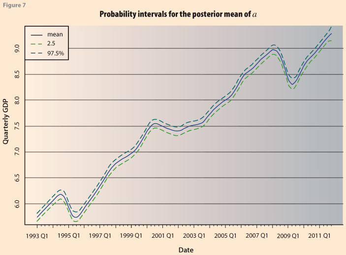
To illustrate further the degree to which the Bayesian estimations agree, or not, with the H-P filter, Figure 8 shows the trend obtained by the Bayesian model and by applying H-P with λ=1600 using the econometric package EViews. They differ very slightly at the end of the series. The important thing here is that the posterior mean of δ (or equivalently λ ) is an estimate of the smoothing constant in the H-P method.

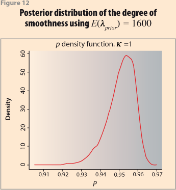
Now we modify the priori distribution for δ and κ by setting (forcing) the mean of the prior distribution to be 1600, the value recommended to use for λ on quarterly data with the H-P filter, i.e. in Bayesian notation E(λ)=1600. This will again allow us to analyze the resulting degree of smoothness as computed from the simulations using expression (10). Since traditionally H-P is applied to seasonally adjusted series we will take as our observed series the INEGI seasonally adjusted Mexican GDP series, see http://www.inegi.org.mx/sistemas/bie/.

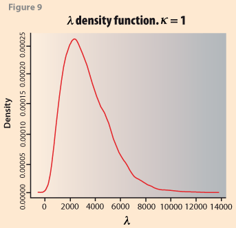
Recalling that if we set the parameter k=1 in the WinBUGS code then λ is directly comparable to δ we run WinBUGS using the seasonally adjusted series as input, with k=1.0 and we obtain that E(λ |y,λ_prior=1600)=3329 a value for λ well within the range of ad-hoc values suggested by Hodrick and

Prescott (1997). This compares well with the previous value obtained without restricting the prior mean, E(λ |y)=2764. Figure 9 shows its posterior distribution and Table 2 the corresponding statistics.

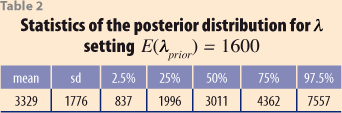
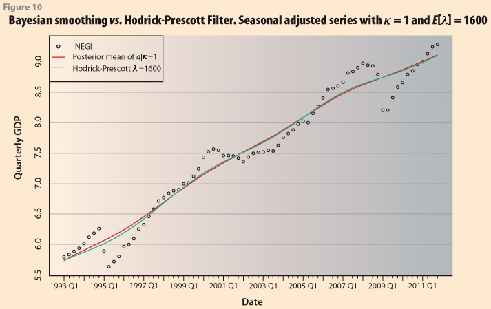
In Figure 10 we compare the two smoothed series from H-P using λ =1600 and the one obtained with the Bayesian procedure restricting the prior mean as E(λ)=1600. As in the previous case, the Bayesian approach has the additional advantage that it is possible to obtain probability intervals for the trend, by using the quantiles of the posterior distribution of the vector α, Figure 11.

Confidence intervals are also obtained in Guerrero (2007), using an unobserved components model. He uses pre-specified smoothness of 60% and λ=0.96. He indicates that "even if the … value of λ has been established by the standard application of the smoothing method (e.g. 1600), we should be aware that the smoothness achieved varies according to the sample size." So that "The basic proposal … is to select the percentage of smoothness at the outset, instead of the smoothing constant." However it is not clear how to choose this percentage.

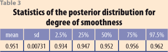
As would be expected, the smoothness in this case is more than when allowing a variable κ. The posterior distribution for the smoothness index is given in Figure 12 and its statistics are provided in Table 3. The posterior mean is 95.1%. If the corresponding smoothness index is obtained for the H-P procedure with λ =1600 it results in a value of 93.08, which is very close.

Final Remarks

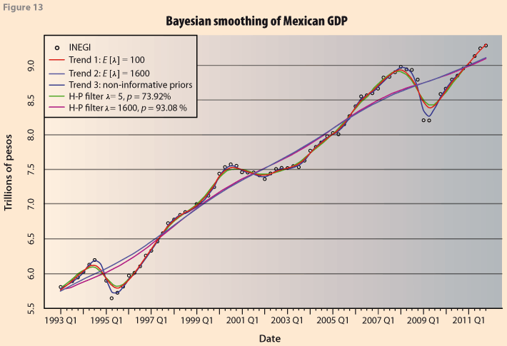
As a final output, Figure 13 shows a ¨summary¨ of the previous results. The main point is that the results from the Bayesian approach provide a natural way for obtaining the smoothing constants. Furthermore, they are obtained with a wealth of additional information that can be used for more thorough analyses. For example it can also be used to obtain the Business Cycles, Heath (2012), and probability intervals for them. This is not done here because it is beyond the scope of the paper. Clearly, using some previously given value, as is done in H-P has many implications for the results (trend, confidence limits, etc.) depending on sample size, and the data themselves.

References

Akaike, H. (1980), "Seasonal Adjustment by a Bayesian Modeling", Journal of Time Series Analysis 1, 1-13.
Burns, A.F. and W.C. Mitchell (1946), "Measuring Business Cycles", NBER Studies in Business Cycles No. 2, New York: Columbia University Press.
Carlin, B.P. (1992), "A Simple Montecarlo Approach to Bayesian Graduation", Transactions of the Society of Actuaries XLIV, 55-76.
de Alba, E. and R. Andrade (2011), "Bayesian Graduation. A Fresh View", ASTIN Colloquium.
Guerrero, V. M. (2007), "Time series smoothing by penalized least squares", Stat. Probab. Lett., 77, 1225-1234.
Guerrero, V. M. (2008), "Estimating Trends with Percentage of Smoothness Chosen by the User", International Statistical Review 76, 2, 187–202.
Guerrero, V.M., Juarez, R. & Poncela, P. (2001). "Data graduation based on statistical time series methods". Stat. Probab.Lett., 52, 169–175.
Heath, J. (2012), "Lo que Indican los Indicadores", INEGI, Mexico.
Hickman, J.C. and Miller, R.B. (1977), "Notes on Bayesian graduation". Transactions of the Society of Actuaries 24,7-49.
Hickman, J.C. and R.B. Miller (1978). Discussion of 'A linear programming approach to graduation'. Transactions of the Society of Actuaries 30, 433-436.
Hodrick, R. J. and E. C. Prescott (1997), "Postwar U.S. Business Cycles: An Empirical Investigation", Journal of Money, Credit and Banking, Vol. 29, No. 1, pp. 1-16.
Kimeldorff, G.S. and D.A. Jones (1967), "Bayesian Graduation", Transactions of the Society of Actuaries 11, 66–112.
Maravall, A. (1993). "Stochastic linear trends. Models and estimators". Journal of Econometrics 56, 5-37.
Maravall, A. and del Río, A. (2007). "Temporal aggregation, systematic sampling, and the Hodrick-Prescott filter". Computational Statistical Data Analysis, 52, 975–998.
Mardia, K.V., J.T. Kent and J.M. Bibby (1989), "Multivariate Analysis", Academic Press.
Schlicht, E. (2005), "Estimating the smoothing parameter in the so-called Hodrick-Prescott filter", Journal of the Japan Statistical Society, 35, 99-119.
Taylor, G. (1992), "A Bayesian interpretation of Whittaker-Henderson Graduation", Insurance: Mathematics and Economics 117-16, North-Holland.
Whittaker, E.T (1923), "On a New Method of Graduations". Proceedings of the Edinburgh Mathematical Society, 41 63-75.

Appendix 1