Early Monthly Estimation of Mexico’s Manufacturing Production Level Using Electric Energy Consumption Data

 

Estimación oportuna mensual del nivel de producción manufacturera en México mediante el uso de datos de consumo de energía eléctrica

 

Daniel Alba Cuéllar and Hugo Hernández Ramos
INEGI, daniel.alba@inegi.org.mx, and hugo.hernandez@inegi.org.mx

Acknowledgements: The authors wish to express their deepest gratitude to former INEGI President Eduardo Sojo Garza-Aldape and current INEGI President Julio Alfonso Santaella Castell for their valuable suggestions in designing the core strategy for building and testing regression models. Special thanks go to Enrique De-Alba-Guerra, INEGI Vice-President, for coming up with the idea of incorporating logarithmic differences into the modeling phase. The authors also wish to thank Arturo Blancas, Head of the Economic Statistics Directorate, Susana Perez, Director of Economic and Agriculture Censuses, and Gerardo Durand, Director of Economic Administrative Registers, for their valuable advice in the realization of this project. The effort from several INEGI colleagues in collecting and organizing the data used in this project is also appreciated. Last but not least, INEGI is deeply indebted to the CFE employees, who have provided Electric Energy Consumption data without failing a single month.

Vol. 12, Núm. 3 - EPUB                                                   Early Monthly... - EPUB

Directly measuring the monthly Manufacturing Production Level in Mexico via national accounting methods is an elaborate process, yielding a preliminary figure approximately 40 days after the end of the reference month. A separate analysis conducted by INEGI (Mexico’s National Statistical Office) showed that in Mexico’s manufacturing sector, there is a significant linear relationship between Electric Energy Consumption and Production Level. Currently, Electric Energy Consumption data from the Federal Electricity Commission (CFE) are made available to INEGI approximately 15 days after the end of the reference month; this timeliness in the availability of CFE data, combined with the observed linear relationship, allowed INEGI to build an econometric model which produces early estimates for the Production Level Index. In this paper we describe the initial analysis conducted by INEGI to build a model which explains the relationship between both variables; then we describe the characteristics and evolution of the “definitive” econometric model, and compare early estimates, computed in real time, against official Production Level figures, as an empirical means for evaluating early estimation accuracy. We observed that 93% of the time, the official figure is located inside the estimation limits, which were computed with a 95% confidence level; this means that, in this case, observed empirical accuracy approached the theoretical confidence level. Finally, in this paper we comment about INEGI’s data sharing experience with CFE and talk about future steps to improve this nowcasting process. Key words: linear regression; nowcasting; macroeconomic indicators; electric energy consumption, manufacturing activity level index.

La medición directa del nivel de producción manufacturera mensual en México por medio de métodos de contabilidad nacional es un proceso elaborado que arroja una cifra preliminar aproximadamente 40 días después del final del mes de referencia. Un análisis realizado por el Instituto Nacional de Estadística y Geografía (INEGI) mostró que en el sector manufacturero del país existe una relación lineal significativa entre el consumo de energía eléctrica y el nivel de producción. Actualmente, los datos de la Comisión Federal de Electricidad (CFE) correspondientes a la primera variable se ponen a disposición del INEGI alrededor de 15 días después del final del mes de referencia; esta oportunidad en la disponibilidad de información de la CFE, combinada con la relación lineal observada, permitió al Instituto construir un modelo econométrico que produce estimaciones tempranas para el Índice de Nivel de Producción. En este artículo, describimos el análisis inicial realizado por este organismo del Estado mexicano para determinar el modelo que explica la relación entre ambas variables; luego, explicamos las características y la evolución del modelo econométrico definitivo y comparamos las estimaciones oportunas, calculadas en tiempo real, contra las cifras oficiales de nivel de producción, a modo de evaluación empírica. Observamos que 93 % de las veces, la cifra oficial se encuentra dentro de los límites de estimación, que se calcularon con un nivel de confianza de 95 %; esto significa que la precisión empírica observada se acerca al nivel de confianza teórico. Finalmente, en este documento comentamos sobre la experiencia de intercambio de datos entre el INEGI y la CFE, y contemplamos posibles pasos futuros para mejorar este proceso de estimación. Palabras clave: regresión lineal; nowcasting; indicadores macroeconómicos; consumo de energía eléctrica; Índice de Nivel de Producción.

Recibido: 20 de mayo de 2020.
Aceptado: 23 de febrero de 2021.

 

1. Introduction

The aggregate Production Level in Mexico’s Manufacturing Sector is a key macroeconomic variable which gives policymakers important clues about the health status of the national economy, given Mexico’s Manufacturing Sector significant contribution to the National Gross Domestic Product. The objective of this paper is to describe the used methodology aimed to investigate the functional relationship between electric energy consumption and production level in Mexico’s manufacturing sector; it is of great interest to know such functional relationship, since the process for measuring the Monthly Manufacturing Production Level Index (IMAI-31-33) by means of national accounting methods is rather elaborate and time-consuming, while the process for measuring the consumption of electric energy in Mexico’s manufacturing sector is faster and more direct. One would hope that if the latter variable is known in a timely fashion, then it would be feasible to obtain, in an economical way, an early estimate of the manufacturing production level, assuming we know the functional relationship between both variables.

Analysis of Monthly data collected by the Federal Electricity Commission (CFE) and by INEGI (Mexico’s National Statistical Office) shows that there is a strong linear relationship between electric energy consumption and production level aggregated at the manufacturing sector level and at national level, so it seems appropriate to use linear regression methods to estimate the functional relationship between these variables. In practice, INEGI obtains, at establishment level, monthly observations for both the consumption of electric energy and the volume of production (industrial activity), although at different moments in time: on the one hand, electric energy consumption data for establishments are provided to INEGI by CFE, approximately 15 days after the end of the reference month, while on the other hand, volume of production data at establishment level are collected, analyzed, processed, and published by INEGI’s System of National Accounts (SNA) in aggregate and preliminary form, approximately 40 days after the end of the reference month; the empirically observed linear relationship between the two variables at the aggregate national manufacturing sector level, coupled with the timeliness of the data provided by CFE, allow INEGI to obtain good early estimates of the production level in Mexico’s manufacturing sector.

Obtaining a regression model to generate good early estimates for the IMAI-31-33 indicator, based on electric energy consumption data, requires fairly long-time series; for the production level in Mexico’s manufacturing sector, INEGI has compiled monthly observations starting from January 1993; thus, as of February 2020, the IMAI-31-33 time series contains more than 27 years of monthly observations; on the other hand, INEGI, with data from CFE, has compiled monthly electric energy consumption observations starting from January 2013; from these CFE monthly observations, INEGI built an electric energy consumption indicator for Mexico’s manufacturing sector, called ICEE (both ICEE and IMAI-31-33 are acronyms in Spanish). Thus, ICEE is a time series with more than 84 monthly observations (7 years of monthly observations). This, of course, means that we cannot use all the available IMAI-31-33 observations for the construction of a regression model if we want to include ICEE as an explanatory variable. Fortunately, now ICEE is long enough to build statistically valid regression models.

This paper is structured as follows: section 2 describes the origin and characteristics of the data used in our analysis; section 3 describes how we prepare our data for the construction of regression models. Section 4 describes the characteristics of some regression models fitted to the prepared data that were available to us back in 2015, when our objective was to arrive at a functional model for generating early estimations (nowcasts) for the IMAI-31-33 indicator as a function of electric energy consumption; we begin with a simple two-variable linear regression model, and then we progress towards models that overcome the deficiencies of their predecessors. Section 5 shows out-of-sample estimates obtained with the models from section 4, and their accuracy assessments by comparing them against officially published IMAI-31-33 values; the evidence shown in sections 4 and 5 will help us select a “definitive” working model to generate subsequent IMAI-31-33 nowcasts. Section 6 shows the complete sequence of IMAI-31-33 nowcasts generated by the “definitive” model selected in section 5, running from August 2015 to February 2020; we compare this sequence of estimated values against officially published IMAI-31-33 values, and comment on the changes the “definitive” model has undergone across time. Finally, section 7 briefly describes INEGI’s data sharing experience with CFE, and discusses possible avenues for future work.

 

2. Origin and characteristics of the data

CFE data

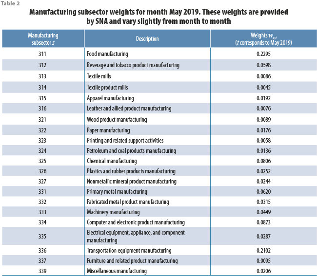
As mentioned above, electric energy consumption data are provided to INEGI by CFE on a monthly basis, approximately 15 days after the end of the reference month; these data contain electric energy consumption values, at user (establishment) level, which start at January 2013. Table 1 shows the structure of CFE monthly data provided to INEGI.

 

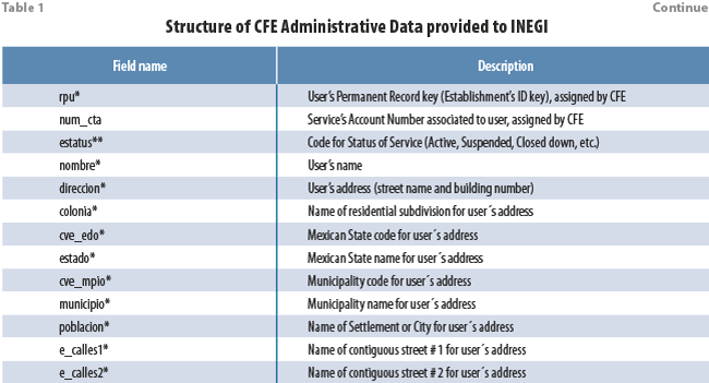
In Table 1, fields with an asterisk (*) at the end of their names are used for record linkage activities, while fields with two asterisks (**) at the end of their names are used for determining which CFE user (establishment) records to include in the sample employed in the computation of the ICEE indicator. Of particular importance is field k_YYYYMM, which in itself contains the electric energy consumption data, in kWh. As of February 2020, INEGI receives each month about five million CFE user records belonging to the industrial (including manufacturing) trade and services economic sectors. Fields k_YYYYMM and i_YYYYMM are available simultaneously in a monthly dataset for several months; CFE sends revised data for all months from the current year and from the previous year, so, for example, CFE data sent after the end of reference month February 2020, contains data for each month of 2019, and data for January 2020 and February 2020.

The record linkage activities (not described in this paper) and the analysis and experiments described below, were conducted by the area of Statistical Linkage of Economic Administrative Registers (DVERA, its acronym in Spanish), which is part of INEGI. The record linkage process allowed DVERA to retrieve the correct North American Industry Classification System (NAICS) code at establishment level from INEGI’s Statistical Business Register (SBR); we’ll see in section 3 why it is important to have the correct NAICS economic-activity-classification code associated to CFE user records. Although the CFE data already contain information on the class of economic activity (field “giro_scian” in Table 1), it has been observed that NAICS classification codes from CFE are in many cases missing or incorrect, since this piece of information is filled in by CFE according to the user’s own declaration when establishing a service contract with CFE. User’s name, business ID from the Federal Tax Agency, and data from address and geographical location fields are used to link CFE records (uniquely identified by their “rpu” keys) to SBR establishment records by means of probabilistic record linkage techniques.

 

Missing values in CFE data

Some Missing values in fields k_YYYYMM and i_YYYYMM are usually observed for the most recent month (i.e., for the reference month). The sooner CFE delivers its monthly data to INEGI, the greater the number of missing values at the reference month; this is probably due to unregistered monthly invoices at the time of data compilation by CFE; this hypothesis is later confirmed when revised CFE data arrives in subsequent months. To fill in missing values, DVERA uses a simple 2-step procedure:

1. For all CFE records r with complete electric energy consumption data in reference month M and previous month M-1, belonging to a given manufacturing subsector S (according to the NAICS classification code from INEGI’s SBR), compute the proportion p_S=∑_r∈Sc_r,M/∑_r∈Sc_r,M-1, where c_r,_M is the electric energy consumption of establishment r at month M. p_s  can be interpreted as an approximation to the monthly growth rate in electric energy consumption for manufacturing subsector S at reference month M.
2. For each record in manufacturing subsector S with missing value c_i,_M, assign c_i,_M = p_Sc_i,_M—1.

NB: This 2-step procedure only takes into account records included in a sample of CFE records especially designed to build the ICEE indicator. Below we give some more details about the construction of this CFE sample.

 

CFE records included in the calculation of the ICEE indicator

Depending on the type of contract that an establishment signs with CFE, its electric energy consumption invoice can be issued once every month, or once every other month; this is indicated by the “tipo_fact” field from Table 1. Large establishments generally receive their CFE invoices (and their consumptions recorded into CFE database) once every month. These large establishments have a high probability of being included in the sample employed for calculating the ICEE indicator, since the main inclusion criterion is to consider those CFE establishments who are statistically linked to a special subset of INEGI’s SBR, called INEGI master sample, which contains the records of the largest establishments in the national economy (the size of an SBR establishment is measured jointly by number of employees and income), and serves as a basis for constructing samples used by INEGI’s national economic surveys. According to data from the 2014 economic census, although large establishments only represent 4% of the total number of establishments in the manufacturing sector, they contribute with 88% of the total income and 68% of the total number of employees in that same sector. As of February 2020, our sample for building the ICEE indicator contains 17,085 CFE records from the manufacturing sector with monthly invoicing frequency; it is worth mentioning that this sample has been growing steadily since we started with this project back in the second half of 2015. When the first early IMAI-31-33 estimate was generated, corresponding to reference month August 2015, our sample for building the ICEE indicator contained 7,744 CFE records. Periodically, CFE data are analyzed by DVERA to update the CFE sample for computing the ICEE indicator by detecting closed down records (which does not necessarily imply that the corresponding establishment has closed down) or new records; these new records sometimes correspond to new establishments and sometimes correspond to existing establishments who updated their contract with CFE. From here on, we can see that CFE data can also be used to periodically update INEGI’s SBR.

 

Complementary electric energy consumption data

In Mexico, there are a few manufacturing businesses who also generate electric energy for self-consumption. Mexico’s Federal Government has an administrative register, at establishment level, for these self-sufficient businesses, which is managed by an agency, very closely related to CFE, called the National Center of Energy Control (CENACE for its acronym in Spanish). Starting from the calculation of the early IMAI-31-33 estimate corresponding to reference month august 2016, we incorporated 43 CENACE records to our CFE sample for computing the ICEE indicator. As of February 2020, our sample includes 66 CENACE records, who represent 1.7% of the total electric energy consumption recorded in our sample across all months. Of course, these 66 CENACE records were also linked to INEGI’s SBR, in order to retrieve their correct NAICS economic activity codes.

 

Data from the System of National Account

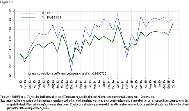
DVERA obtains production level data for manufacturing industries in Mexico directly from the Manufacturing Production Level Index, IMAI-31-33. This indicator, aggregated at the economic sector level, is published on a monthly basis by the System of National Accounts of Mexico (SNA) at the INEGI website. Since the construction process for the IMAI-31-33 indicator by the SNA depends on survey-collected data, it is published approximately 40 days after the end of the reference month. For the manufacturing sector in Mexico, we initially observed that the linear correlation coefficient between ICEE and IMAI-31-33 is high, close to positive 1 (see figure 1); from this point, we see that it is feasible to have a good notion, several days in advance, about the magnitude of the next monthly “true” published IMAI-31-33 value, by using CFE electric energy consumption data, along with a properly built regression model.

NB: In this paper we work only with non-seasonally adjusted time series; this choice, in our experience, produces better results, as we have seen after several exercises with linear regression models involving both non-seasonally adjusted and seasonally adjusted time series. If we want to obtain a seasonally-adjusted nowcast for IMAI-31-33 as a function of electric energy consumption, we can simply append our non-seasonally adjusted nowcast to the non-seasonally adjusted IMAI-31-33 time series itself, and then use a seasonally adjusting software, such as x-13arima-seats.

3. Data preparation to conduct a regression analysis

With the data provided by CFE and SNA, monthly data on electric energy consumption and on volume of production, respectively, are available for the main manufacturing industries in Mexico. From these data, it is possible to build two monthly frequency time series:

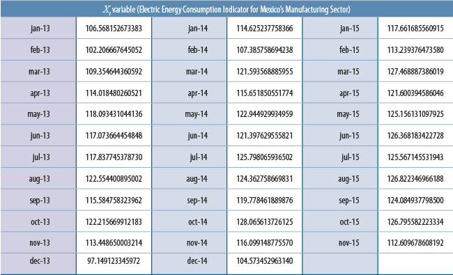
• Time series X_t: electric energy consumption index for Mexico’s manufacturing sector (ICEE).
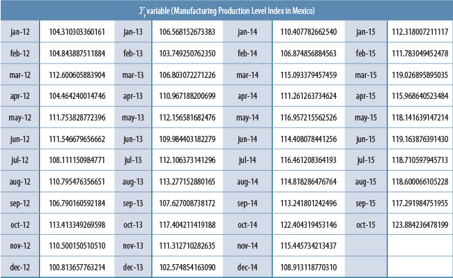
• Time series Y_t: production level for Mexico’s manufacturing sector.

Here, subscript t indicates the month to which a measurement for any of these two variables corresponds.

The Y_t variable is simply a subset of the IMAI-31-33 time series^[1] mentioned above, which can be located within the IMAI file: Original series - Physical volume indices, base 2013 = 100, namely in the row labeled as “31-33 - Industrias manufactureras”. This file can be directly downloaded on the following link (in Spanish): https://bit.ly/3f9PKST

To generate variable X_t from CFE data, the following procedure was defined:

1. For each month t, sum the weighted electric energy consumption values corresponding to all CFE records in our sample:

s_t=∑_rw_s(r),_t c_r,t;

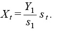
c_r,t is the electric energy consumption (in kWh) of establishment r within our sample in month t, while w_s(r),_t  is a weight that depends both on month t, and on the manufacturing subsector of economic activity s(r) to which establishment r belongs t. Weights w_s,_t  satisfy the convexity property; i.e., the sum of all weights for a fixed month  equals 1. Table 2 shows typical values for weights w_s,_t.

2. Re-scale time series s_t so that it coincides with Y_t at a base period (say t = 1):

    

 

Manufacturing subsector weights w_s,t, just like the IMAI-31-33 indicator, are also provided by SNA; furthermore, their availability coincides with that of the IMAI 31-33 indicator; that is, weights w_s,t are available approximately 40 days after the end of the reference month. In order to estimate the manufacturing subsector weights for the reference month (say, month M) for which electric energy consumption data are already available, but not yet for the IMAI 31-33 indicator, take the most recent weight w_s,M-1 for manufacturing subsector s, and multiply it by the factor w_s,M-12/w_s,M-13, which represents the monthly growth rate that weight w_s,t experienced a year before reference month M; in this way, we have:

where  is an estimate for weight w_s,M.

The data (X_t, Y_t) used in the analysis presented in sections 4 and 5 of this paper correspond to the data available to us back in the second half of 2015, when our objective was to build a “definitive” working model useful in explaining the relationship between X_t and Y_t and at the same time useful in generating “nowcasts” for Y_t. Thus, we have 34 monthly observations available for our present analysis:  t = 1 corresponds to January 2013, t = 2 corresponds to February 2013, ..., t = 34 corresponds to October 2015. Figure 1 shows the time series corresponding to variables X_t and Y_t. Additionally, the values of these two variables are listed in appendix 1 of this document, for the sake of experiment reproducibility. 

 

4. Models fitted to the analysis variables

Once the analysis variables X_{t ,} Y_t are prepared, the objective now is to generate “nowcasts” of  Y_t  as a function of X_t for reference month t = M. To reach this aim, we chose to use linear regression models, commonly used in econometrics. This section describes the main models that we progressively fitted to the analysis variables  X_t and Y_t, indicating in each case their characteristics. When we conducted this model construction exercise, back in 2015, our approach was to progressively find a regression model such that subsequent models improved upon the deficiencies found in its predecessors. This model construction exercise was done with help of the R Statistical Computing Software [2].

 

4.1 Simple linear regression model

The first model fitted to our data was a simple linear regression model of the form

                                     Y_t = α + βX_t + ε_t.                                              (1.0)

For a model of the form (1.0) to be considered as an adequate fit to the data (X_t, Y_t ), in theory the disturbances  ε_t must follow a white noise process; i.e., ε_t variates must be independent and identically distributed, each with normal distribution with mean zero and constant variance σ²; to abbreviate, we denote this requirement as ε_t ~iid N(0, σ²). By using the data in appendix 1 to fit a model of the form (1.0) via Ordinary Least Squares (OLS), we obtain the estimation equation:

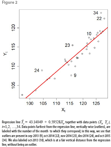
Ŷ_t = 43.14049 + 0.59528X_t;

thus, the estimated parameters are intercept â=43.14049 (5.103), slope =0.59528 (0.043); figures in parentheses indicate standard errors. From here, it is possible to see that both coefficients are statistically significant. Additionally, adjusted R²=0.852, and the corresponding F-test of overall significance has a p-value of  5.1 × 10^-15. Model residuals r_t=Y_t- Ŷ_t (sample estimates of the ε_t disturbances) appear to be approximately centered around 0 (min= -4.3, median= -0.04, max= 5.3). All these model hypothesis tests indicate a good fit so far.

The corresponding fitted regression line is shown in Figure 2, along with data points (X_t, Y_t) used to build model (1.0).

 

Before accepting this model as the definitive one, additional tests are necessary to verify that the residuals r_t come from a white noise process. The Durbin-Watson (DW) test for the fitted model of the form (1.0) gives a test statistic equal to 1.11, with a p-value close to zero; this strongly suggests that we must reject the null hypothesis which states that the model residuals are serially uncorrelated; from this point, we conclude that there is strong evidence that the model residuals r_t follow a 1^st order autoregressive process. To correct the problem of auto-correlated residuals in a linear regression model, there are several alternatives: one is to apply the Cochrane-Orcutt correcting procedure to model the disturbances using a first-order autoregressive model of the form ε_t=ρε_t-1 + v_t, with v_t ~iid N(0, σ²). A second alternative is to use generalized least squares together with the autoregressive structure of the ε_t disturbances (Cochrane-Orcutt uses OLS). A third option is to incorporate explanatory lagged variables X_t-1, Y_t-1 into the regression model; this third approach is known as auto-regressive modeling with distributed lags. For more information about these approaches, see [3].

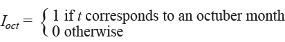
An additional problem with this simple linear regression model (1.0) fitted to our data has to do with the outliers shown in Figure 2. As can be seen, outliers manifest themselves at different months, and for almost 3 years of monthly data values, there are outliers at October (outliers 22 and 34; 10 is not an outlier, but it is not either one of the closest points to the regression line). This suggests the need to add to subsequent linear regression models an indicator variable for the month of October as an explanatory variable; this indicator variable could be roughly defined as:

4.2 Autoregressive model with distributed lags

If the disturbances from regression model (1.0) follow a first-order autoregressive process ε_t = ρε_t-1 + v_t, with v_t ~iid N(0, σ²), which appears to be the case when fitting model (1.0) to our data, then it is possible to correct this autoregressive effect if we instead use a model of the form:

                                Y_t − ρY_t-1 = α (1− ρ) + ß (X_t − ρX_t-1) + v_t,                (2.0)

which is obtained by subtracting ρY_t-1 = αρ + βρX_t-1 + ρε_t-1 from model (1.0). Of course, p corresponds to the autocorrelation coefficient which characterizes the 1^st order auto-correlated disturbances from model (1.0). The Cochrane-Orcutt procedure obtains an estimate of p using an iterative algorithm, although it is also possible to re-parameterize model (2.0) in order to obtain an autoregressive model with distributed lags of the form:

                                Y_t = α* + ρY_t-1 + ß X _t + γ* X _t-1+ v _t,                          (2.1)

where α* represents the quantity α(1- ρ), and γ* represents the quantity -ρβ. The parameters from model (2.1) can be estimated via OLS.

By fitting a model of the form (2.1) to the data shown in appendix 1 via OLS, together with an indicator variable I_oct, we obtained the following estimation equation (note that, in this case, for variables X_t, Y_t and I_oct, the initial value t for corresponds to February 2013):

Ŷ_t = 12.54 + 0.69Y_t-1 + 0.52X_t − 0.33X_t-1 + 5.21I_oct. 

It is possible to see that all regression coefficients in fitted model (2.1) are statistically significant; adjusted R² = 0.948, and model residuals appear to be centered at zero (min = -2.6, median = 0.3, max = 2.0).

The Durbin-Watson test for fitted model (2.1) yields a test statistic equal to 2.44, with an associated p-value close to 0.3. From this point, we see that fitted model (2.1), which includes an indicator variable for October, is free of residual first-order autocorrelation, and all its explanatory variables are statistically significant.

Additionally, a Breusch-Pagan test for heteroscedasticity (non-constant variance) was conducted on the model residuals, producing a test statistic equal to 0.716 with an associated p-value close to 0.4; The Breusch-Pagan test’s null hypothesis states that there is no heteroscedasticity in the residuals; The p-value in this case tells us that there is not enough evidence to reject the null hypothesis, so it is concluded that fitted model (2.1) successfully passes the heteroscedasticity test.

Another test that can be done on the residuals from the fitted model with form (2.1) is that of Cramér-von Mises, to verify the normality of the residuals. In this case, we obtained a test statistic equal to 0.0502, with associated p-value close to 0.5. In the Cramér-von Mises test, the null hypothesis states that the residuals are normally distributed; the p-value indicates that we cannot reject the null hypothesis, so it is concluded that the residuals from model (2.1) are normally distributed.

When working with linear regression models which contain two or more explanatory variables, as is the case with model (2.1), we must make sure that there is no high linear correlation among explanatory variables; for this, we applied a multicollinearity test (for more details, see [4]), obtaining Variance Inflation Factors (VIFs) equal to 7.6, 1.2 and 8.2; if any VIF is greater than 10, then we have multicollinearity problems, which does not occur in this case. Therefore, fitted model (2.1) does not have multicollinearity problems.

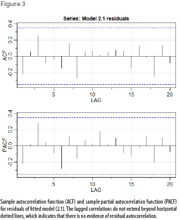
Finally, the graphs for the sample autocorrelation function (ACF) and for the sample partial autocorrelation function (PACF), shown in Figure 3, confirm that the residuals from fitted model (2.1) are uncorrelated over time.

From this point, we see that fitted model (2.1) is adequate, although it could be argued that it has several estimable parameters, and a couple of VIF’s are rather large. Next, we’ll investigate a more parsimonious alternative.

4.3 Logarithmic differences model

A proposed modeling alternative to that presented in subsection 4.2 is the logarithmic differences model, which is built by means of the following expression:

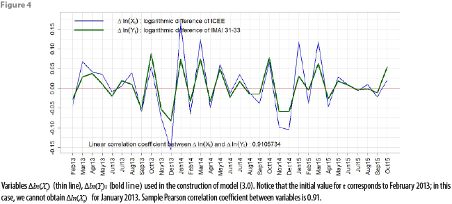
                                        Δln(Y_t) = ßΔln(X_t) + ɛ_t,                    (3.0)

where Δln(Y_t): = ln(Y_t) - ln(Y_t-1) = ln(Y_t/Y_t-1) is the logarithmic difference of Y_t, Δln(X_t): is the logarithmic difference of X_t, β is the parameter to be estimated (via OLS), and ε_t are the usual stochastic white-noise disturbances in a linear regression model. The advantage of this model lies in its parsimony; that is, it is not necessary to estimate many  parameters, unlike model (2.1). Note that this model does not directly estimate values for Y_t; instead, it estimates the monthly growth rate of Y_t. To see this, first note that ln (1 ± r) ≈ ± r if r is a reasonably small value; for example, ln (1+0.05) = 0.04879 ≈ 0.05, while ln (1 + 0.05)= -0.05129 ≈ -0.05. Now, the logarithmic difference Δln(Y_t) = ln(Y_t/Y_t-1) is in fact the natural logarithm of the variation of Y_t with respect to its previous monthly value Y_t-1; if this monthly growth is reasonably small, then Y_t/Y_t-1 will be of the form 1+r; for example, if Y_T 118.1, Y_T-1 = 116.0, for t = T, then Y_T/Y_T-1 = 1.018103 = 1 + 0.018103, which means that when t = T, Y_t grows, or varies 1.8%, with respect to its previous monthly value Y_t-1; note that in this example, Δln(Y_T) = ln(Y_T/Y_T-1) = 0.01794153 is reasonably close to the true Y_t monthly growth rate for t = T.

Figure 4 shows a graph of the transformed variables Δln(X_t) and Δln(Y_t), obtained directly from the data in appendix 1.

 

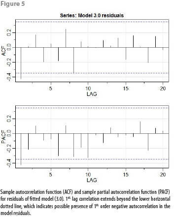
By fitting, via OLS, a model of the form (3.0) to the data represented graphically in Figure 4, together with an indicator variable for the months of October, we obtained the estimation equation = 0.523002  Δln(X_t) + 0.47991 I_oct. We also applied the same battery of tests from subsection 4.2 to the fitted model (3.0), without the multicollinearity test. We found out that fitted model (3.0) successfully passes all tests, except for the Durbin-Watson test, as can also be seen from Figure 5. 

 

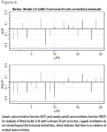
To correct this 1st. order autocorrelation problem, we applied the Cochrane-Orcutt correction procedure, originally defined in [5], to fitted model (3.0); in this way, we obtained the estimation equation   = 0.547802 Δln(X_t) + 0.043357 I_oct, with residual term , where = 0.4277 ( is used to correct model coefficients). This time, all tests on this corrected model (3.0) are successfully passed, getting an adjusted R² equal to 0.93 and no autocorrelation problems on model residuals, as Figure 6 shows.

 

We conclude that fitted model (3.0) with Cochrane-Orcutt correction passes all our criteria for obtaining an adequate linear regression model. In the next section we’ll test empirically the out-of-sample forecasting accuracy of the models obtained here. The results from this section and the next will help us to decide on a “definitive” model.

 

5. Comparisons of out-of-sample estimates among regression models

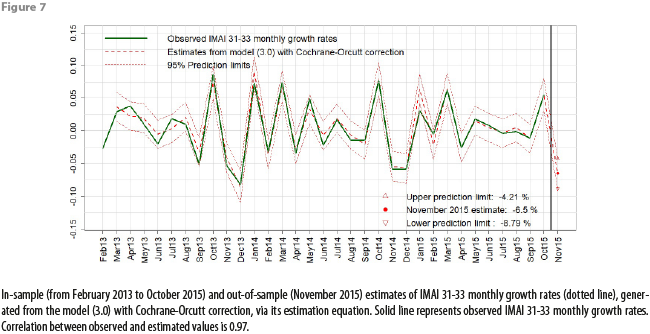
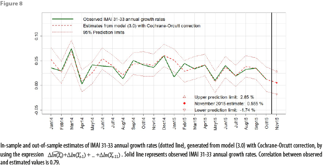
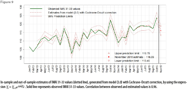
In this section we compute out-of-sample estimates using the models built in section 4 and then compare such estimates against officially published values. As we previously saw, the data used to build our models span the time interval from January 2013 to October 2015; therefore, circumscribing ourselves to the data from appendix 1, we have the November 2015  X_t value as the only element for producing out-of-sample estimates for Y_t values. Thus, in order to “nowcast” the November 2015 IMAI 31-33 value, we incorporate the November 2015 ICEE value (namely, 112.61) into the estimation equations obtained in section 4. It is worth mentioning that the models described in section 4 were originally built on December 9, 2015, and their predictions for the month of November 2015 were compared against the “observed” November 2015 value for the IMAI 31-33 indicator, published on January 11, 2016 as a preliminary figure (namely, 117.5659). Additionally, with the published IMAI 31-33 figures, we obtained the observed (or “true”) annual and monthly growth rates: the observed annual growth rate of the IMAI 31-33 indicator for November 2016 is 100(Y_nov2015/Y_nov2014 - 1) = 100(117.5659/115.4457 - 1) = 1.84 (see appendix 1 for Y_nov2014 value). Likewise, the observed monthly growth rate of the IMAI 31-33 indicator for November 2016 is 100(Y_nov2015/Y_oct2015 - 1) = 100(117.5659/124.2666 - 1) = -5.39. Note that in the calculation of the observed monthly growth rate, we are using the revised figure for the October 2015 IMAI 31-33 indicator (124.2666) instead of the corresponding Y_oct2015 value found in appendix 1 (123.8842).

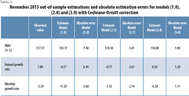
We’ll use these observed values as part of an additional criterion for assessing the models built in section 4. Table 3 shows out-of-sample estimations from models (1.0), (2.1) and (3.0) along with their corresponding absolute errors with respect to observed values.

 

 

Appendix 3 explains how the estimated values in table 3 were computed.

Estimation errors shown in table 3 indicate us that the logarithmic differences model (3.0) with Cochrane-Orcutt correction produces the most accurate November 2015 IMAI 31-33 nowcasts. From the model diagnostics and hypothesis testing procedures described in section 4, we see that both the distributed lags model (2.1) and the logarithmic differences model (3.0) with Cochrane-Orcutt correction have desirable statistical properties, although model (2.1) has more estimable parameters than model (3.0) and could potentially be more unstable as new monthly observations become available. We then conclude that, from the models built in section 4, the logarithmic differences model (3.0) with Cochrane-Orcutt correction is the most parsimonious, robust and is the one which produces the most accurate forecasts; thus, we select model (3.0) as our “definitive” model.

Figures 7, 8, and 9 show graphs for in-sample and out-of-sample estimations produced with our definitive model, using the data from appendix 1. The in-sample estimations for IMAI 31-33 values and for annual growth rates were obtained by applying the same expressions derived in appendix 3.

 

 

  

 

6. Evaluating logarithmic differences model in real time

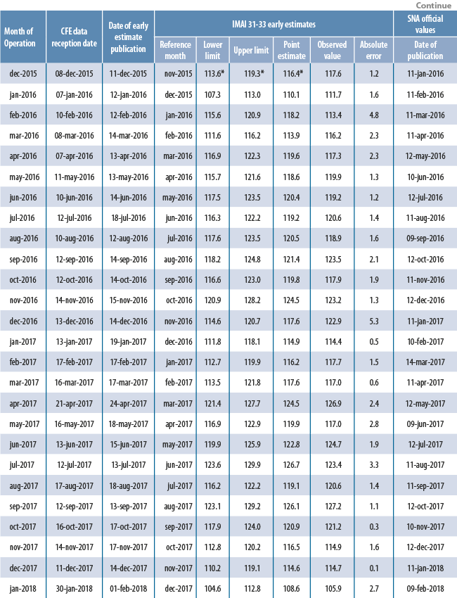
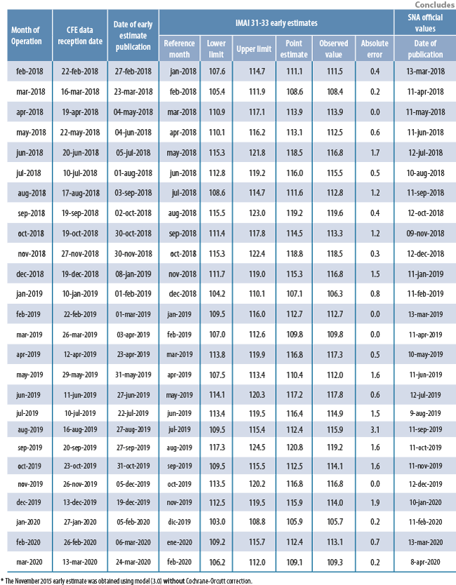
Having decided on what model to use in order to generate subsequent nowcasts for the IMAI 31-33 indicator, DVERA has fitted, on a monthly basis, linear regression models of the form (3.0) to produce such nowcasts, beginning at reference month August 2015, and verifying each time that the fitted logarithmic differences model passes all the statistical tests for model adequacy. Figures 10, 11, and 12 show the comparisons of IMAI 31-33 nowcasts against published IMAI 31-33 values. It is worth mentioning that these comparison graphs are updated each month, appending each new time an additional estimate and corresponding observed value, published as a preliminary figure (no revised figures for officially published IMAI 31-33 values are displayed in Figures 10, 11 and 12). Appendix 2 shows a table with dates for reception of CFE data, calculation of nowcasts, and official publication of IMAI 31-33 values.

 

  

 

 

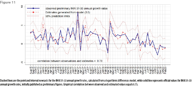
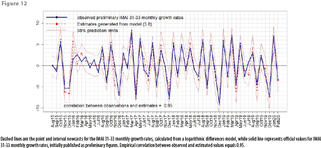
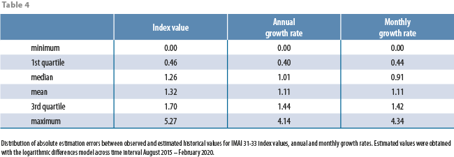
Table 4 shows the distribution of absolute errors between observed and estimated historical values. From Table 4 and from Figures 10, 11, and 12, we can see that for any month in the time interval August 2015 – February 2020, magnitudes of absolute estimation errors are similar across the 3 estimated quantities: index values, annual and monthly growth rates. For most months, the officially published value has “landed” inside the 95% prediction intervals, which have a mean width of between 5 and 6 percentage points for any of the 3 estimated quantities (this means that, with 95% confidence, our point estimates have a maximum associated error of ±3%). Table 4 shows that, empirically, absolute errors tend to group around 1; a very few times, the absolute error has been close to 0, and a very few times, it has been large. In fact, only 4 times the observed IMAI 31-33 value has landed outside the 95% prediction interval: in January 2016, in November 2016, in June 2017 and in July 2019. This means, that, empirically, officially published values have landed inside the prediction intervals 92.7% of the time, which is close to the theoretical (or nominal) 95% confidence level incorporated into prediction intervals.

 

As can be seen from Figure 10, there was a change in the base year for the IMAI 31-33 indicator between September 2017 and October 2017; before that change, the IMAI 31-33 indicator average for the year 2008 was 100.00; after the change, the IMAI 31-33 indicator average for the year 2013 is now 100.00. Basically, this only translates as a rescaling of the IMAI 31-33 indicator; our procedure for estimating monthly growth rates via a logarithmic differences model is unaffected by this change in SNA methodology for constructing the IMAI 31-33 indicator. Note that  values from appendix 1 correspond to published IMAI 31-33 values under the 2008 base year.

 

Evolution of the logarithmic differences model (3.0)

The model chosen for producing successive IMAI 31-33 nowcasts has basically retained its initial form across time interval August 2015 – February 2020; the only modifications we have done to this “definitive” model consist in gradually adding (as needed) indicator variables for modeling significant seasonal effects, similar to the I_oct  indicator variable. The logarithmic differences linear regression model for producing the February 2020 IMAI 31-33 estimates has the following functional form:

ΔlogY_t = ß₁ΔlogX_t+ ß₂I_aug+ ß₃I_oct+ ß₄I_nov+ ß₅I_jan+ ɛ_t,

where ΔlogY_t  and ΔlogX_t are the respective logarithmic differences for response and explanatory variables Y_t and X_t at month t, as explained in section 4;  ε_t follows a first order autoregressive process which is corrected via the Cochrane-Orcutt procedure. As of reference month February 2020, the estimation equation is:

ΔlogY_t = 0.5467ΔlogX_t+ 0.0184I_aug + 0.0420I_oct + 0.0265I_nov+ 0.0149I_jan

We compared statistical tests outputs among all fitted logarithmic differences models of the form (3.0) across months and found out that the common estimated coefficients (for variables ΔlogX_t  and I_oct, and for coefficient p) have small variance. This is empirical evidence that the relationship between variables X_t, Y_t is structurally stable across time, independent of business cycles. 

 

7. INEGI’s data sharing experience with CFE, conclusions and future work

The monthly data on electric energy consumption that CFE transmits to INEGI are packed into 16 files, each corresponding to one of the 16 regions in which CFE divides the Mexican territory. Transmission of CFE data to INEGI is usually made two weeks after the end of the reference month; sometimes, however, due to technical or administrative difficulties, CFE data have been transmitted to INEGI a few days later than usual. Overall, there have been no months during the realization of this project in which no data has been received from CFE; this has enabled the successful realization of an empirical evaluation, in real time, of early IMAI 31-33 estimates. In appendix 2, we can see the dates on which INEGI has received data on electric energy consumption from CFE, and the comparison between early IMAI 31-33 estimates and published IMAI 31-33 values. It is important to emphasize that the agreement between INEGI and CFE to share information is rather informal, since a memorandum of understanding (MoU) has not been signed yet. As of this date, INEGI and CFE relationship continues to be cordial, and both institutions are working in the elaboration of a proper MoU.

The IMAI 31-33 nowcasts, generated from August 2015 to February 2020 with the help of a logarithmic differences model relating manufacturing production level to electric energy consumption at national level, have been communicated to some Federal Government Agencies in Mexico, such as the Central Bank of Mexico (BANXICO), the Mexican Social Security Institute (IMSS), The Office of the Treasury and Public Credit (SHCP), the Tax Administration Service (SAT), CFE itself, and some other key users within INEGI. Each month, right after generating nowcasts for the IMAI 31-33 indicator, DVERA prepares an official letter with a technical annex, which is sent to the INEGI Presidency, responsible for disseminating the results to other Federal Government Agencies. This official letter clearly states that the results obtained are of an experimental nature. As of the writing of this article, INEGI is studying the possibility of publishing these results on its website, under the category of experimental statistics.

 

Some concluding remarks and possible lines for future work

By processing monthly electric energy consumption data from the majority of large manufacturing establishments in Mexico, we have produced an electric energy consumption index that has a significant linear relationship to the Monthly Manufacturing Production Level in Mexico. This enables INEGI to produce nowcasts for Mexico’s Manufacturing Production Level, given the timeliness in the availability of electric energy consumption data. The monitoring in real time of such nowcasts for the last four years has provided empirical evidence in favor of the structural stability of the relationship between electric energy consumption and production level in Mexico’s manufacturing sector. In order to improve the quality of the IMAI 31-33 nowcasts, DVERA is working continually to keep an updated sample of large manufacturing establishments, and is monitoring the evolution of the variables involved, in order to update the “definitive” model if the need arises.

As future work, INEGI is contemplating the possibility of adding an additional explanatory variable to the “definitive” model; specifically, the explanatory variable considered is the monthly production of vehicles in Mexico’s automotive subsector; these data are collected jointly by the Mexican Association of the Automotive Industry (AMIA) and by INEGI. It has been observed that this monthly variable, which is updated only 10 days after the end of the reference month, has a high linear correlation with the IMAI 31-33 indicator. Preliminary exercises to build regression models with IMAI 31-33 as the response variable, and ICEE and the production of vehicles as explanatory variables, have already been carried out.

References

^[1] Sistema de Cuentas Nacionales de México. Cuentas de Corto Plazo y Regionales: Fuentes Metodológicas. 20 de Agosto de 2013. INEGI. Link (in Spanish, accessed on August 14, 2019): https://bit.ly/3tdVK57

^[2] The R project for statistical computing: https://www.r-project.org/

^[3] Davidson, R., & MacKinnon, J. G. (1993). Estimation and inference in econometrics. OUP Catalogue. Oxford University Press, number 9780195060119

^[4] Kutner, M. H.; Nachtsheim, C. J.; Neter, J. (2004). Applied Linear Regression Models (4th ed.). McGraw-Hill Irwin

^[5] D. Cochrane & G.H. Orcutt (1949). Application of Least Squares Regression to Relationships Containing Auto-Correlated Error Terms. Journal of the American Statistical Association. Volume 44, Issue 245: pages 32–61.

 

Appendix 1. Data used in the construction of regression models

Appendix 2. Dates on reception of CFE data and production of early estimates; evaluation of early estimates for IMAI 31-33 values

Appendix 3. Formulas for computing nowcasts using the models described in section 4

Model (1.0): the estimation for the November 2015 IMAI 31-33 value, Ŷ_t, was obtained by simply using the corresponding estimation equation, together with the X_t value for November 2015 from appendix 1; the estimation for the corresponding annual growth rate was computed by using the formula 100(Ŷ_t/Y_t-12-1), while the corresponding monthly growth rate was computed with the formula 100(Ŷ_t/Y_t-1-1); note that we must use the values from appendix 1 to compute the estimates for annual and monthly growth rates, since they are computed in real time; i.e., before the published revised figures Y_t-12 and Y_t-1 are available.

Model (2.1): the estimation for the November 2015 IMAI 31-33 value, Ŷ_t, as in the case of model (1.0), was obtained by using the corresponding estimation equation, together with the needed values Y_t-1, X_t and X_t-1 from appendix 1. The corresponding estimations for the annual and monthly growth rates were obtained using the same procedure as in the case of model (1.0).

Model (3.0) with Cochrane-Orcutt correction: unlike models (1.0) and (2.1), in this case we are directly estimating the November 2015 IMAI 31-33 monthly growth rate from the corresponding estimation equation; for this we need to plug in the values X_nov2015 and X_oct2015 from appendix 1; note that in this case, I_oct=0. Now, to estimate the corresponding annual growth rate, we first note that log(Y_t/Y_t-12) acts as an approximation to the annual growth rate of Y_t, in the same way log(Y_t/Y_t-1) acts as an approximation to the monthly growth rate of Y_t; we also observe that:

logY_t −logY_t-12 = logY_t -logY_t-1 +logY_t-1 -logY_t-2 +⋯+logY_t-11 -logY_t-12

or equivalently,

log(Y_t/Y_t-12) =∆ln(Y_t )+∆ln(Y_t-1)+⋯+∆ln(Y_t-11).

From this last expression, it seems reasonable to approximate the annual growth rate of Y_t for November 2015 by using the sum

where  is the output from the estimation equation, and the quantities ∆ln(Y_t-1),∆ln(Y_t-2),…,∆ln(Y_t-11) can be computed from the data in appendix 1. This is precisely the procedure we used to estimate the annual growth rate from model (3.0) shown in table 3.

Finally, it is also possible to compute an estimation for the IMAI 31-33 indicator from the quantity ; just solve for Y_t in expression ln(Y_t)-ln(Y_t-1)=∆ ln(Y_t):

ln(Y_t)=∆ ln(Y_t)+ln(Y_t-1)

Y_t=e^{∆ ln(Y_t)+ln(Y_t-1)}

Y_t=Y_t-1 e^∆ln(Y_t).

From this last expression, it seems reasonable to approximate Y_t by using

We used this last expression to estimate the IMAI 31-33 value from model (3.0) shown in table 3.

^[1] For the construction of IMAI-31-33, SNA uses information mainly from INEGI’s Monthly Survey on Manufacturing Industries (EMIM for its acronym in Spanish); this national-level economic survey is also based on INEGI’s SBR master sample. See [1] for more information.